Chun-Yi Lee · portfolio · 1 min

Pick the method the data structure calls for

Three public manufacturing datasets, three different data structures, three deliberately different strategies — not one technique applied three times.

LayerDatasetStructureMethod
L1SECOM one wafer = a static snapshot imbalanced classification + drift monitoring
L2PHM 2016 CMP one wafer = an in-process trajectory time-series virtual metrology
L3Bosch one product = a path across stations process flow graph + attribution
What came out of it: a single finding that ties all three together — drift is not automatic. It is what happens to the part of the process you did not measure.
The through-line

Does what I learned still hold next month?

SECOM — no

Weekly fail rate falls 23% → 1–5% over three months. 55–66% of sensors exceed the PSI action threshold in every test segment. And a walk-forward simulation shows no retraining policy beats leaving the model frozen — detecting drift is not the same as being able to fix it.

Bosch — no, seductively

A path's historical fail rate ranks first of 263 features by importance — and still degrades out-of-time ranking. Train-vs-test correlation: Spearman ρ = 0.09 (p = 0.36).

PHM CMP — yes

Error does not grow with tool wear. The most-worn quartile is the most accurate, because consumable usage is an input feature the model already learned.

The difference is not model class. It is whether the degradation axis was itself measured and fed to the model.
L1 · SECOM · 2 min

Rare bad wafers, and a factory that keeps moving

Problem. 590 sensors per wafer, 6.6% fail. An escaped bad wafer costs ~100× a needless re-inspection. Rank wafers so limited re-inspection capacity lands where failures are.

SPC first. A fab engineer reaches for a control chart, so that is the bar: Hotelling T² on PCA scores catches 8% of failures at 11% false alarms. Failures are not global multivariate outliers — which is what justifies supervised ML.

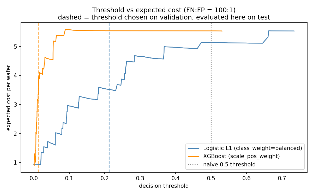
Threshold from cost, never 0.5. The operating point is the minimum of the expected-cost curve, chosen on a validation window inside training.
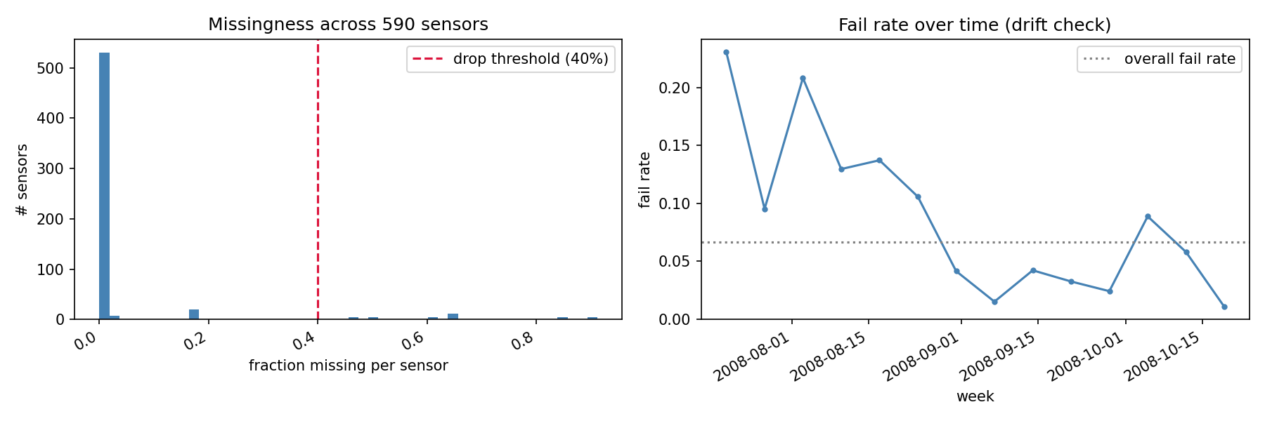
55–66%
of sensors past the PSI 0.25 action band, in every test segment
Expected cost per wafer against decision threshold for two models
Cost-optimal thresholds sit at 0.01–0.21, nowhere near the 0.5 default.
Sensor missingness histogram and weekly fail rate over three months
The yield ramp: the model is calibrated to a factory that no longer exists by the time it is scored.
L1 · SECOM · the negative result

The control that stopped me reporting a fake win

I built the sensor correlation network with the standard fMRI functional-connectivity recipe — correlate all pairs, keep the strongest 5% of edges, rank by degree centrality — then tested whether hub sensors make better features than mutual-information top-k.

And against randomly chosen subsets of the same size.

Neither principled method beats random at any k. Both sit inside ±1 sd of the random control everywhere. Nothing beats keeping all 444 features.

Without the random control this slide would have said "network hubs beat mutual information at k=20" — and been wrong. The k=50 mutual-info spike is matched by the random control's own spike at k=80.

Honest label: this is a data-driven correlation network, not a process flow graph. SECOM's sensors are anonymized. The process-flow story is Bosch's.
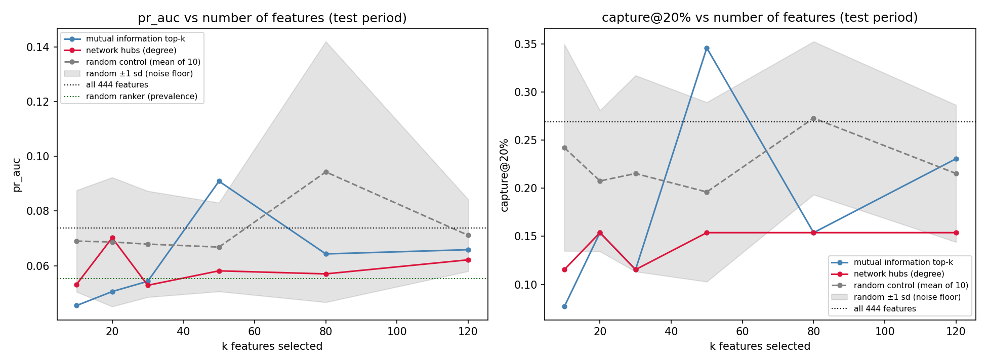
PR-AUC and capture@20% against number of features for three selection methods
Grey band = ±1 sd across 10 random subsets. It swallows both principled methods.
L1 · SECOM · testing my own claim

I argued retraining would fix the drift. Then I measured it.

This sub-project was built around the argument that under drift, a monitor-and-retrain loop matters more than model choice. So I wrote the experiment that tests it: walk forward through the wafer stream, compare four policies at identical windows, refit preprocessing, model and threshold on every retrain.

policyPR-AUCretrains fails in trainp vs frozen
frozen0.093 063—
triggered (PSI fires)0.088 7790.30
expanding0.0888 790.30
sliding0.0548 330.47

No policy beat frozen. And that −41% on sliding is not a finding — one window with 5 failures carries 75% of it. Paired window by window: 3–4, p = 0.47.

The reportable result is that this dataset cannot answer the question — 41 failures across 8 windows will not separate four policies. I rewrote the sub-project's conclusion rather than keep a claim the experiment failed to support.

What it did establish: the PSI trigger fires in 7 of 8 windows, so "retrain when drift is detected" is operationally the same as "retrain always" — the trigger buys no economy here.
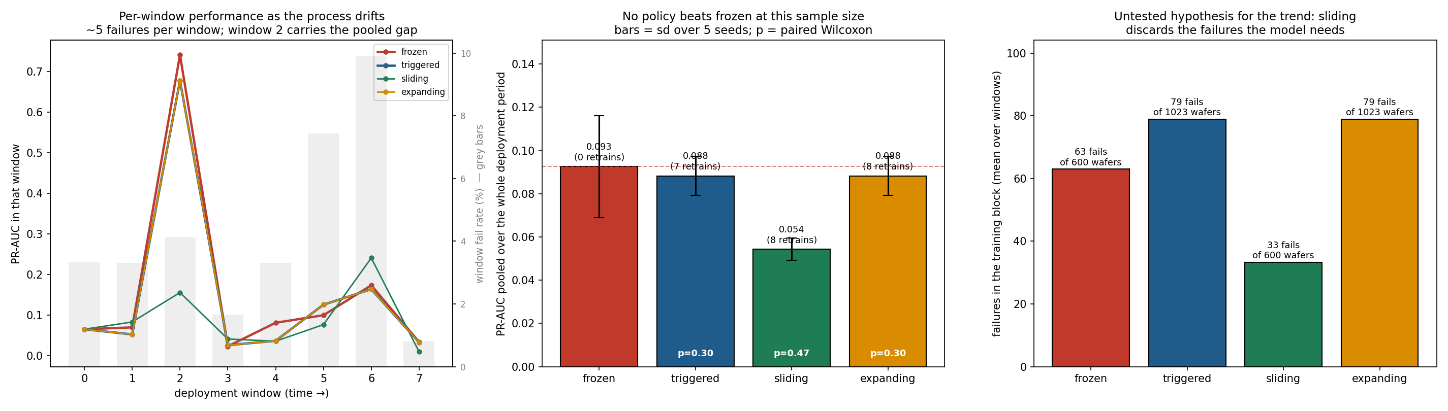
Per-window performance, pooled comparison with p-values, and failures per training block for four retraining policies
Left: window 2 is the whole story. Middle: error bars overlap and no p clears 0.30. Right: the untested mechanism — 33 vs 63 vs 79 failures to learn from.
L2 · PHM 2016 CMP · 3 min

Virtual metrology: measure fewer wafers, catch bad polish sooner

Problem. Measuring material removal rate is slow and occupies metrology capacity, and the answer arrives after the run. If the in-process trace predicts it, most wafers skip physical measurement.

The data was supposed to be gone. phmsociety.org now 404s its own download links and the official test labels ship as ?. I recovered the trajectories from the Internet Archive and found the withheld test labels published separately — 424 (WAFER_ID, STAGE) keys matching the official test set exactly. So this is scored on the real competition test set, not a holdout I invented.
MSE 6.24
MAE 1.82 · R² 0.993 · official 424-run test set
The deflated number. MRR is bimodal; separating the two clusters is easy and inflates R². Within the main cluster it is R² 0.897, MAE 1.93. That is the number I quote.
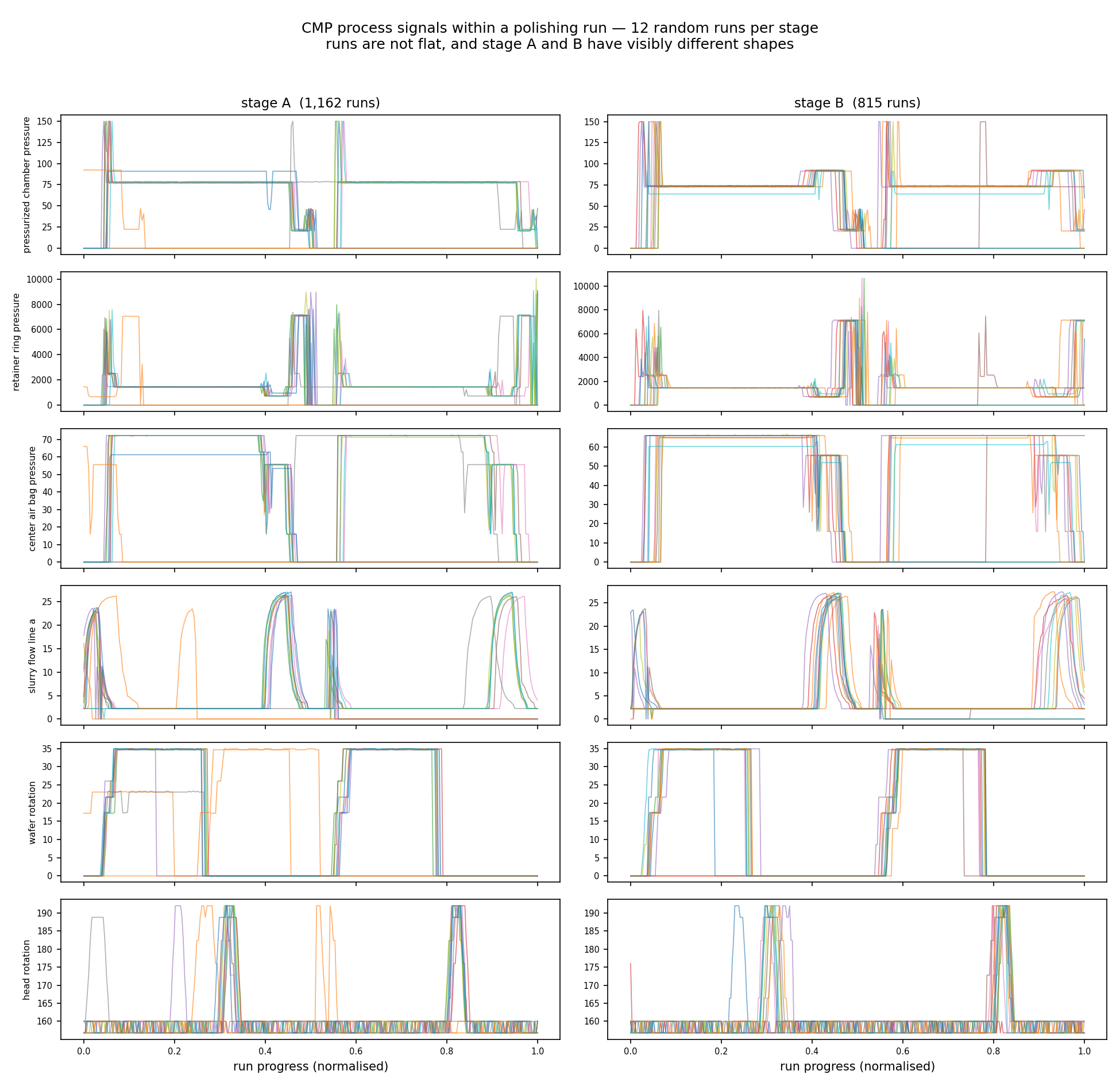
Six process signals across twelve runs each for stage A and stage B
Multi-phase polishing recipes with distinct step structure — this is why L2 is a time-series problem and not another table.
L2 · PHM CMP · the hypothesis that failed

Tool ageing did not degrade the model — and that is the finding

The expectation: as the polishing pad and dresser wear, prediction error grows, motivating a retraining trigger on accumulated hours.

Polishing-table wearn MSEMAE
Q1 fresh106 8.932.16
Q2106 5.271.79
Q3106 7.431.90
Q4 worn106 3.321.44

The most-worn quartile is the most accurate. Consumable usage is an input feature, so the model learned the wear effect rather than decaying with it.
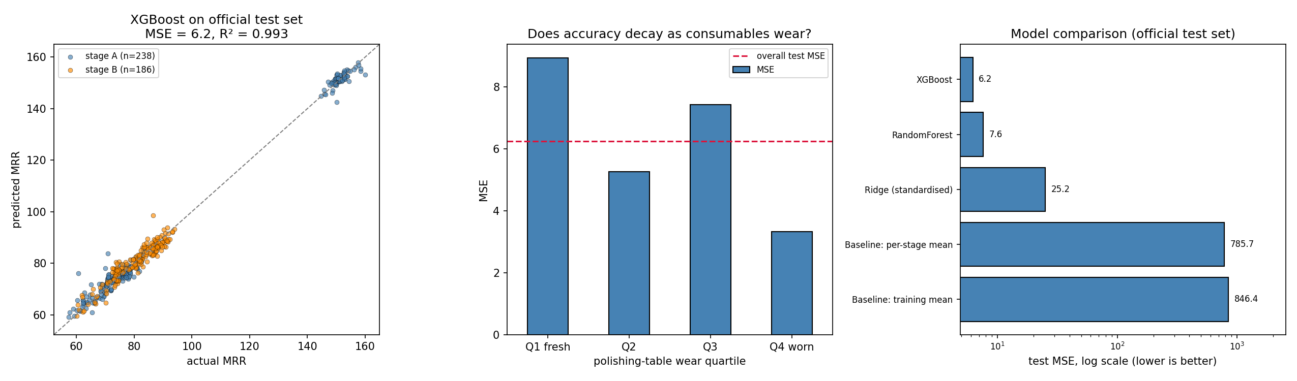
Consequence for production. The retraining trigger here should watch for operating conditions outside the trained range — new recipes, usage beyond the observed span — not accumulated hours.
Predicted vs actual MRR, error by wear quartile, and model comparison
L2 · PHM CMP · hand-crafted vs learned

The deep model that won on validation and lost on test

Same split, same official test set, same metric, same static inputs. Only the trajectory encoding differs: ~200 hand-crafted time and frequency descriptors, versus a network reading the raw signals.

modeltrackval MSE test MSE
XGBoosthand-crafted31.98 6.24
RandomForesthand-crafted29.57 7.64
BiGRU ×3 seedslearned27.63 14.45
Ridgehand-crafted44.47 25.17
1D-CNN ×3 seedslearned 18.0128.59

Hand-crafted wins by 2.3×. At ~1,600 training runs, compressing a trajectory into physically-motivated descriptors beats asking a network to rediscover them.
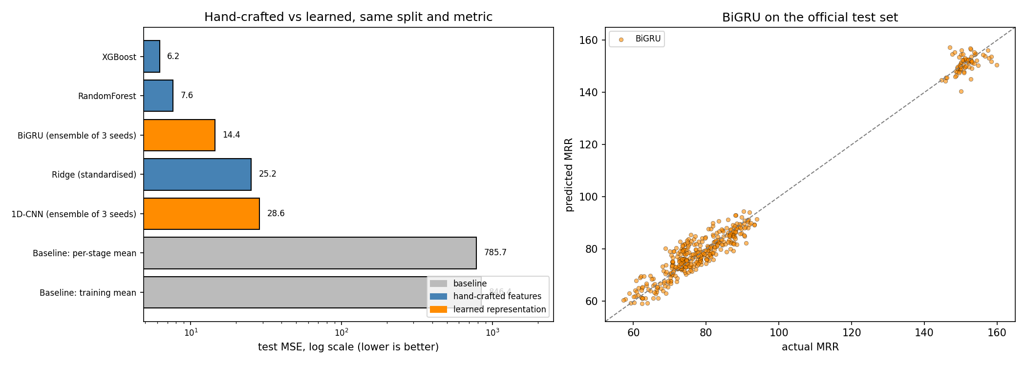
Look at the 1D-CNN row. Best validation MSE of any model, worst test MSE of any non-baseline model — the ranking inverts. Its seed spread is 26.7–39.8, a 49% swing, against the GRU's 14.9–15.8. Select on validation, report one seed, and you ship the worst model believing it is the best.
Test MSE by model and track, and BiGRU predictions against actual MRR
The answer is not a preference between methods. It is a sample-size argument.
L3 · Bosch · 3 min

From predicting failures to locating them

Nothing in the data says the stations are connected. Column names (L3_S36_F3939) encode line and station; date columns encode the order a product visited them. Those two together are the edge list.
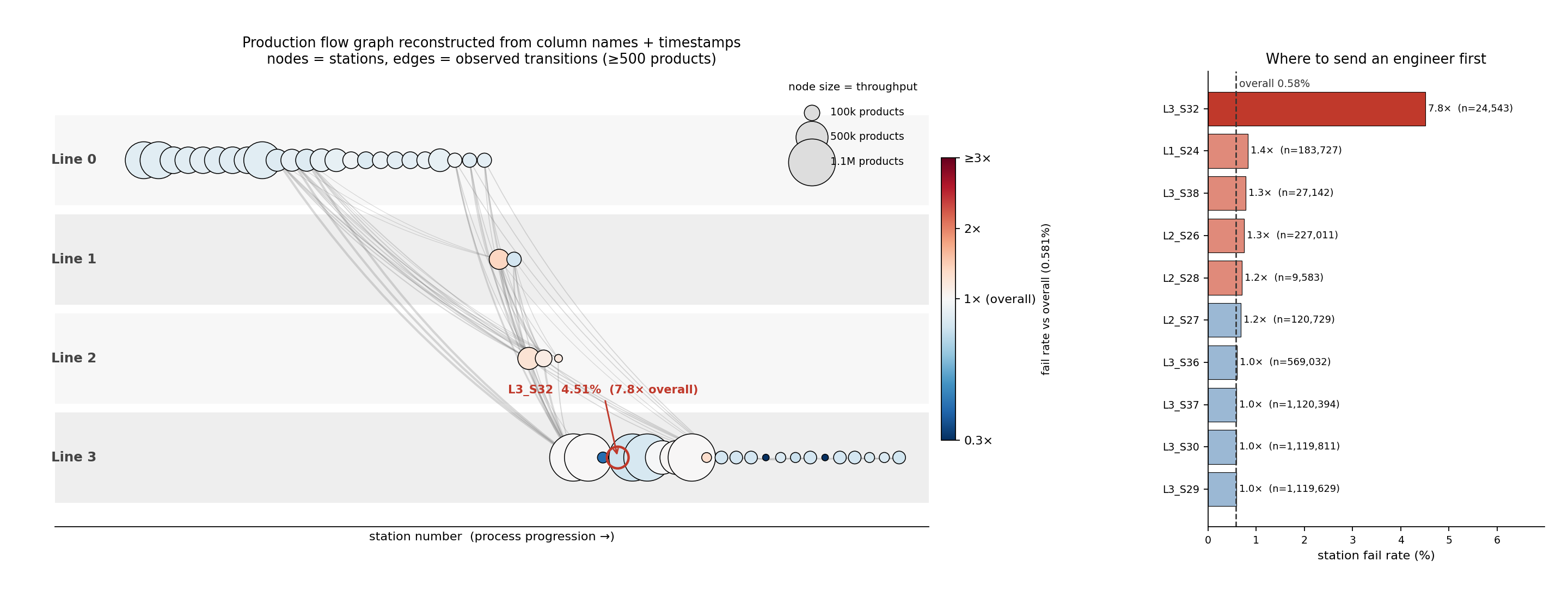
Reconstructed Bosch production flow graph with a ranked station fail-rate panel
52 stations · 243 transitions · 7,927 production paths, rebuilt from 1.18M products.
7.8×
L3_S32 fails at 4.51% vs 0.58% overall, across 24,543 products. No other station exceeds 1.5×.
1.28%
fail rate for products routed L1_S24 → L3_S29, skipping the L2 inspection stations — roughly double the 0.67% of the otherwise identical route through L2_S26.
Honest framing: Bosch is automotive, not semiconductor. It is the public dataset whose schema encodes a complete production-line structure. A fab's process flow has the same shape, so the method transfers even though the parts do not.
L3 · Bosch · the SPC bar

Why the control chart cannot work on a 7,927-route plant

Before claiming ML is needed, run the chart a process engineer reaches for. Hotelling T² compares a unit's measurement vector against an in-control mean and covariance — which presumes every unit is measured the same way.

With 7,927 distinct routes, most measurement slots are empty for most products. Those blanks are stations never visited, not readings that went missing. Imputing them invents in-control behaviour that never happened.

baselinerecall @UCL false alarmsPR-AUC vs random
T², all products, imputed46.1% 35.9%0.0047 1.2×
T², largest route family6.5% 5.2%0.0051 1.5×
XGBoost model A—— 0.02446.2×
The naive chart's 46% recall is an illusion — it comes from alarming on more than a third of all good products. Restricted to the one route family where the assumption genuinely holds, T² manages 1.5× random.

SPC's failure here is structural, not statistical. The plant does not have one process to chart. It has 7,927 — which is exactly the argument for modelling the routing explicitly.
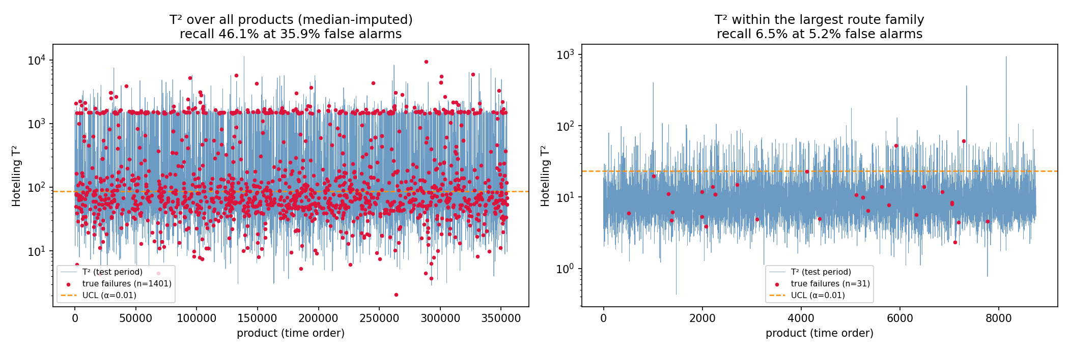
Hotelling T-squared control charts over all products and within the largest route family
Red = true failures. Left: imputation pushes the whole population past the limit. Right: legitimate but blind.
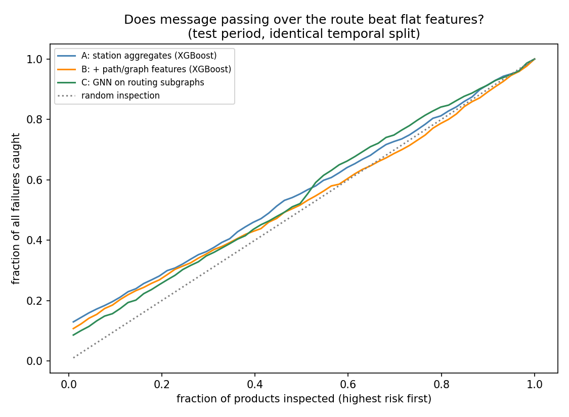
Capture curves for the two XGBoost variants and the GNN
All three models track each other; the graph structure does not separate them.
L3 · Bosch · the result I am proudest of

The graph features looked like a 43% win. They were not.

modelMCC @valMCC @oracle PR-AUCcapture@20%
A: station aggregates0.069 0.1120.024 0.287
B: + path & graph features0.099 0.1020.018 0.272
C: GNN on routing subgraphs0.062 0.0950.018 0.260

MCC needs a threshold. At the oracle threshold — the best any of them could reach on test — the model without graph features wins, and every threshold-free metric agrees. path_risk still ranked first of 263 features by gain.

Model C injects the structure a completely different way — each product becomes a subgraph of stations it visited, so message passing can combine a reading with its neighbours' along the route. It lands with B, behind A. Two independent routes to the same answer.

Why: a path family's historical fail rate does not carry forward. Across 108 families with ≥200 products in both windows, Pearson r = 0.23, Spearman ρ = 0.09 (p = 0.36), while prevalence drifts 0.66% → 0.40%. The encoding memorised a level, not a property.
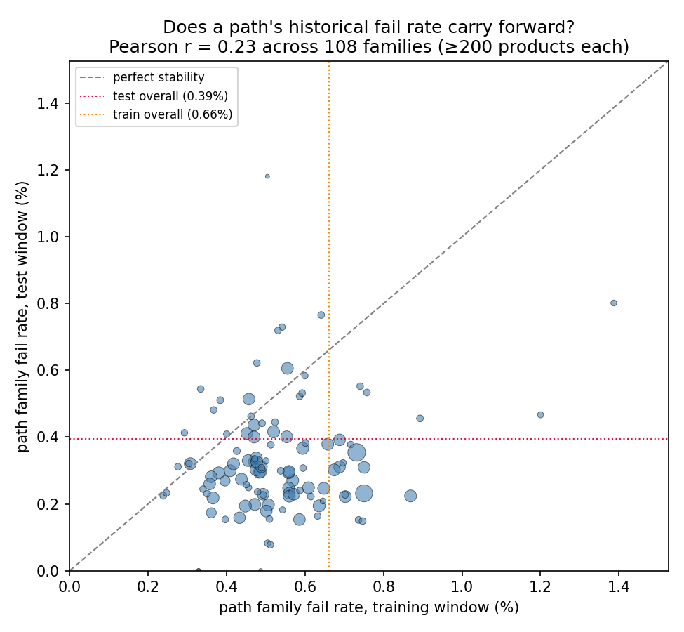
Feature importance measures what a model leaned on — not whether leaning helped. The process graph earns its keep as an attribution instrument, not a feature generator. Which is fine: attribution is what the fab actually wants.
Path family fail rate in the training window against the test window
Below the diagonal is the yield ramp; the absent trend is the instability.
Engineering & discipline

What I refused to do

Leakage red lines

  • No random splitting of timestamped data — all three datasets drift.
  • No oversampling outside the CV loop.
  • No statistic fit on data the model shouldn't see — imputers, scalers and target encodings are all fit on the training window.
  • A wafer's stage A and stage B runs never straddle a split (asserted in code, not assumed).

No accuracy, anywhere

"All pass" scores 93% on SECOM and 99.4% on Bosch. Reported instead: PR-AUC, MCC, expected cost under an asymmetric matrix, and decile capture — because inspection capacity is the real constraint.

No magic features

Public Bosch solutions reach MCC ≈ 0.4+ largely through row-Id ordering, which leaks the response. Excluded. My numbers are what the process data supports.

Scale handled honestly

4.7 GB across ~2,100 sparse columns: read in 100k-row chunks and collapsed to per-station aggregates before anything is held at once. Missing values are routing information ("never visited this station"), preserved as visit counts and left as NaN — never imputed.

Shared, tested foundations

common/ holds metrics, splits, SPC baselines and drift monitoring, used by all three sub-projects. 20 unit tests, including one that catches an int64 overflow in the MCC threshold search at scale.

Close · 1 min

What I would say to a process engineer tomorrow

Actionable now

  • Go look at station L3_S32. 4.51% fail rate, 7.8× the floor average, on 24,543 units.
  • Re-examine the routing policy that lets products skip the L2 inspection stations — those routes fail at double the rate.
  • Deploy CMP virtual metrology on the routine population (MAE ≈ 2% of the value) and keep physical metrology for the tails.
  • Do not ship a SECOM model without the monitor. The drift trigger fires in every test segment; a rolling retrain matters more than model choice.

The transferable habit

Every one of these projects has a place where the obvious reading of the numbers was wrong:

looked truethe check
graph features lift MCC 43%oracle threshold
hub selection beats mutual inforandom control
virtual metrology R² 0.993within-cluster fit
error grows with tool wearstratified error table
the 1D-CNN is the best modelheld-out test + seed spread
sliding retrain is 41% worsepaired Wilcoxon per window
retraining fixes drift — my own claim walk-forward simulation

Each cost one extra diagnostic. None of them needed a bigger model. The last one cost me my own headline claim, which I rewrote rather than defended. That is the habit I would bring to a yield team.

Cross-domain note, kept short: the network analyses come from fMRI functional connectivity — correlate channels, threshold, rank by degree centrality. Same mathematics, different network. The transferable part is knowing when a correlation structure is worth treating as a graph, and being willing to conclude that it is not.