Semiconductor Quality ML — Structure-Driven Method Selection
Three public manufacturing datasets, three data structures, three deliberately different strategies. The claim this portfolio makes: method choice should follow data structure, not fashion.
| Layer | Dataset | Data structure | Strategy | Headline result |
|---|---|---|---|---|
| L1 static | SECOM | one wafer = one static snapshot | imbalanced classification + drift monitoring | drift dominates: fail rate falls 23%→2% over 3 months, retraining trigger fires in every test segment |
| L2 temporal | PHM 2016 CMP | one wafer = an in-process time trajectory | time-series virtual metrology (regression) | MSE 6.24 / MAE 1.82 on the official competition test set |
| L3 graph | Bosch | one product = a path across stations | process flow graph analysis + GNN | station L3_S32 fails at 7.8× the overall rate; graph helps attribution, not prediction |
The finding that ties the three together
All three ask the same question in the end — does what I learned still hold next month? — and they answer it differently, which is the actual thesis:
- SECOM: no. Both the labels and the features move. But a walk-forward deployment simulation shows no retraining policy beats leaving the model frozen — and says why: 41 failures across 8 windows cannot resolve four policies. Detecting drift is not the same as being able to fix it.
- Bosch: no, and seductively so. A path's historical fail rate ranks first by feature importance and still degrades out-of-time ranking (Spearman ρ = 0.09 between train and test windows).
- PHM CMP: yes — because the degradation axis (consumable wear) is an input feature, so the model learned it instead of decaying with it. Error is lowest in the most-worn quartile.
Drift is not automatic. It is what happens to the part of the process you did not measure.
The second thread: six times the obvious reading was wrong
Including, at the bottom of the table, this repo's own headline claim.
Each sub-project has a place where the numbers said one thing and a single extra diagnostic said another. Those diagnostics are the actual work.
| what looked true | the check | what was true |
|---|---|---|
| Graph features lift Bosch MCC 43% | MCC at the oracle threshold | Plain tabular ranks best; the gain was threshold luck. A GNN, added independently, agrees |
| Network-hub feature selection beats mutual information on SECOM | Random subsets of the same size | Neither beats random at any k; nothing beats keeping all 444 features |
| CMP virtual metrology reaches R² 0.993 | Fit within the main MRR cluster | R² 0.897 — the bimodal label distribution was inflating it |
| Model error grows as CMP tooling wears | Error stratified by wear quartile | It does not; the most-worn quartile is the most accurate |
| The 1D-CNN is the best CMP model (best validation MSE of all) | Held-out test + seed spread | Worst test MSE of any non-baseline model; 49% swing across seeds |
| Sliding-window retraining is 41% worse than frozen (pooled PR-AUC) | Paired per-window Wilcoxon | One window with 5 failures carries 75% of that gap; window-by-window it is 3–4, p = 0.47. Nothing is significant |
| Retraining under drift will recover performance — this repo's own original claim | Walk-forward simulation of four policies | It does not, measurably. The dataset cannot resolve the question, and saying so beats picking the flattering number |
Reading order
→ Start here: jamesleecy.github.io/semiconductor-quality-ml
| ▶ 10-minute deck | 12 slides; arrow keys to navigate, P to print |
| 📄 Full report | all six write-ups, figures and tables in one page |
| TALKING_POINTS.md | interview index, every claim traced to a script |
| 產業技術報告 | technical report in Traditional Chinese for process/yield engineers and manufacturing DS teams — results, deployment considerations and limitations |
| 白話技術文件 | plain-language explainer in Traditional Chinese — everyday analogies, no prior ML knowledge assumed |
Those two HTML pages are served by GitHub Pages, so the links render as
pages rather than source. python build_report.py regenerates the report
from the READMEs, which stay the single source of truth.
Shared engineering principles (enforced in every sub-project):
- Business framing first — every README opens with the problem and a cost number, not a dataset description.
- Cost asymmetry — thresholds derived from expected-cost curves, never 0.5.
- SPC before ML — Hotelling T² / EWMA / CUSUM baselines first.
- No leakage — temporal & group-aware splits; imputation/scaling/oversampling fit inside training folds only.
- Explainability → actionability — every analysis ends in "what should the engineer do next", not an AUC.
- Drift & retraining — each sub-project defines PSI/KS monitoring and a retraining trigger.
Layout
common/          # shared metrics, splits, SPC baselines, drift monitoring
01_secom/        # L1: imbalanced classification (UCI SECOM)
02_phm_cmp/      # L2: virtual metrology regression (PHM Society 2016)
03_bosch/        # L3: process flow graph + GNN (Kaggle Bosch)
tests/           # unit tests for common/
reports/         # rendered HTML/PDF reports
slides/          # interview deck
Status
| milestone | state |
|---|---|
| M0 shared modules + tests | done (20 tests) |
| M1 SECOM | done |
| M2 Bosch graph + attribution + ablation | done |
| M3 PHM CMP hand-crafted feature track | done |
| M4 sensor network · sequence models · GNN · SPC | done |
| M5 talking points · deck · HTML report | done |
Setup
pip install -r requirements.txt
python -m pytest tests/ -q
Each sub-project downloads its own data (*/download_data.py) and is
reproducible end to end; see its README. Bosch needs a Kaggle API token.
Data and licence
The code is MIT licensed. No dataset files are included here. SECOM (UCI), PHM 2016 CMP (PHM Society) and Bosch Production Line Performance (Kaggle) are fetched by the download scripts and remain under their original providers' terms — including Kaggle's competition rules, which require accepting them before the Bosch data can be downloaded.
Method-transfer note: the network analyses (sensor correlation networks, station-graph centrality) transfer directly from fMRI functional-connectivity / degree-centrality work — same math, different domain.
半導體製造異常偵測與良率預測 — 技術報告
作者:李俊毅 (Chun-Yi Lee) 對象:製程/良率工程師、製造資料科學團隊、智慧製造技術主管 程式與完整結果:https://github.com/JamesLeeCY/semiconductor-quality-ml
本報告假設讀者熟悉晶圓製造、SPC 與良率管理。若需入門版本, 請看 白話技術文件。
摘要
本專案以三份公開製造資料,各自對應一種資料結構層次,驗證「依資料結構 選方法」的判斷,而非以單一演算法套用三次。三個案例分別得到可行動的結論:
| 層次 | 資料 | 任務 | 關鍵結果 |
|---|---|---|---|
| L1 靜態 | SECOM | 不平衡分類 | 漂移主導;四種重訓策略皆未勝過凍結模型,且資料量不足以分辨 |
| L2 時序 | PHM 2016 CMP | 虛擬量測迴歸 | 官方測試集 MAE 1.82(≈2%),具備取代日常實體量測的精度 |
| L3 圖 | Bosch | 流程圖歸因 | L3_S32 站不良率為整體 7.8 倍;圖的價值在歸因而非預測 |
三個案例共同指向一個結論:
漂移不是必然發生的,它是「未被量測的那部分製程」所產生的結果。 CMP 案例中,耗材使用量是模型輸入之一,模型因此學會了磨損效應而非被其 侵蝕;SECOM 與 Bosch 的退化軸未被量測,兩者皆在時間外推上失效。
對產線的直接意涵:與其追求更複雜的模型,不如先確認退化軸是否已被感測器 涵蓋並納入特徵。
1. 方法論框架
三個案例共用同一套規範,這部分比模型選擇更決定結果可信度。
1.1 防資料洩漏(三條紅線)
| 紅線 | 具體作法 |
|---|---|
| 不得隨機切分 | 三份資料皆有時間戳且皆存在漂移,一律採時間切分 |
| 不得跨單位切分 | CMP 以 wafer 為分組單位,同片晶圓的 stage A/B 不得分屬訓練與測試(程式中以 assert 驗證) |
| 統計量不得偷看 | 補值中位數、標準化參數、目標編碼一律僅由訓練視窗計算 |
實務上的落差可量化:文獻中 SECOM 的高分多半來自隨機切分, 該落差本身即為洩漏幅度。本專案在誠實切分下的成績明顯較低,這是預期內的。
1.2 指標選擇
全專案禁用 Accuracy。SECOM 不良率 6.6%、Bosch 0.58%,全判良品即可得到 93.4% 與 99.4%。採用的指標與其產業意義:
| 指標 | 產業意義 |
|---|---|
| PR-AUC | 稀有事件下的排序能力(取代易被大量負例灌水的 ROC-AUC) |
| capture@20% | 每班僅能複檢 20% 產品時,可攔截多少比例的不良 — 最貼近產能限制 |
| 預期成本 | 以成本矩陣把混淆矩陣換算成金額,使門檻成為商業決策 |
| MCC | Bosch 競賽官方指標,需先定門檻 |
| MSE | PHM 競賽官方指標 |
1.3 成本不對稱與門檻決策
漏檢(不良流出)與誤殺(良品複檢)的代價差距,SECOM 設 100:1、Bosch 設 50:1。所有分類門檻由預期成本曲線推導,並在訓練期內部的驗證視窗選定後 凍結,不使用 0.5 預設值。
SECOM 的成本最佳門檻落在 0.01–0.21,與 0.5 相距甚遠;直接採用預設值會 使成本數倍上升。
1.4 SPC 基準線先行
任何 ML 模型上場前先建立 SPC 基準,理由是現場工程師的第一反應必然是 「用管制圖不就好了」。必須先量化管制圖的極限。
2. L2 — CMP 虛擬量測(產業價值最高)
2.1 問題與價值
CMP 的材料移除率(MRR)量測慢、佔用量測產能,且結果在製程完成後才取得。 若能由製程中感測器軌跡即時推估 MRR,可釋放量測產能並提前攔截異常研磨。
2.2 資料與方法
- 1,981 次研磨、672,744 筆軌跡列、19 個具物理意義的製程訊號 (研磨壓力、漿料流量、晶圓/研磨台/修整器轉速、耗材使用量等)
- 每次研磨壓縮為 208 個長度不變特徵:時域(水準、離散、極值、趨勢斜率、 偏態、峰度、端點)與頻域(頻譜重心、低頻能量占比、頻譜熵)
- 切分:以 wafer 分組 + 時間排序
2.3 結果(官方競賽測試集,424 次研磨)
| 模型 | 測試 MSE | MAE | R² |
|---|---|---|---|
| 全體平均(基準) | 846.4 | 21.7 | 0.00 |
| Ridge | 25.17 | 3.67 | 0.970 |
| RandomForest | 7.64 | 1.94 | 0.991 |
| XGBoost | 6.24 | 1.82 | 0.993 |
| BiGRU(3 種子集成) | 14.45 | 2.80 | 0.983 |
| 1D-CNN(3 種子集成) | 28.59 | 3.23 | 0.966 |
MRR 實際範圍 57–160,MAE 1.82 約為 2% 誤差。
關於評估基準的說明:本競賽於 2016 年結束後未公開測試集答案,官方檔案 中該欄位皆為
?。本專案自 Internet Archive 取回軌跡資料,並自另一來源 取得測試集真值(424 筆(WAFER_ID, STAGE)鍵值與官方測試集 100% 吻合), 因此上述成績為在真正的競賽測試集上評分,非自訂 holdout。
2.4 兩個必須誠實揭露的限制
其一,R² 被雙峰分布灌水。 MRR 明顯分為約 75 與約 150 兩群,區分兩群本身 容易。僅計算主群(MRR < 120,佔 351/424)時 R² 為 0.897、MAE 1.93, 此為反映實際量測精度的數值。
其二,手工特徵顯著優於深度序列模型。 在 n≈1,600 的訓練量下,XGBoost (6.24)優於 BiGRU(14.45)達 2.3 倍。更值得注意的是:1D-CNN 的驗證集 MSE 為全體最佳(18.01),測試集 MSE 卻為所有非基準模型中最差(28.59), 排序完全顛倒,三個種子間離散度達 49%。
實務啟示:在千級樣本量下以驗證集挑選深度模型並回報單一種子結果, 極可能交出最差的模型。本專案兩種架構皆採三種子集成並回報離散度。
2.5 機台老化分析:與預期相反
依研磨台使用量四分位分層檢視誤差:
| 磨損程度 | n | MSE | MAE |
|---|---|---|---|
| Q1 最新 | 106 | 8.93 | 2.16 |
| Q2 | 106 | 5.27 | 1.79 |
| Q3 | 106 | 7.43 | 1.90 |
| Q4 最舊 | 106 | 3.32 | 1.44 |
誤差未隨磨損上升,最磨損分位反而最準。 原因是耗材使用量本身即為模型 輸入特徵,模型已學會磨損效應。
對重訓練政策的意涵:此製程的重訓練觸發條件應設定為 「出現訓練範圍外的操作條件」(新配方、使用量超出已觀測區間), 而非「累積運轉時數」。
3. L3 — Bosch 製程流程圖歸因
框架說明:Bosch 為汽車零件產線,非半導體。採用原因是其欄位命名完整 編碼了產線結構,為唯一可示範流程圖方法的公開資料。晶圓廠 process flow 結構同構,方法可直接遷移。
3.1 流程圖重建
資料本身未提供站點連接關係。結構來自兩處:
- 欄位命名:
L3_S36_F3939→ 產線 3、站點 36、特徵 3939 - 時間戳欄位:產品通過各站的先後順序即為有向邊
由 118 萬筆產品重建出 52 個站點、243 條轉移、7,927 條生產路徑, 每件產品中位數通過 13 站。
3.2 歸因結果(可直接行動)
| 發現 | 數值 | 建議行動 |
|---|---|---|
| L3_S32 站異常 | 不良率 4.51%,為整體 0.58% 的 7.8 倍,涵蓋 24,543 件 | 優先派工程師稽核該站;其餘 51 站無一超過 1.5 倍 |
| 路由政策風險 | 跳過 L2 檢查站的路線(L1_S24 → L3_S29)不良率 1.28%,為經過 L2_S26 之相同路線 0.67% 的約 2 倍 | 檢視允許跳站的排程規則 |
3.3 SPC 在多路徑產線的結構性失效
Hotelling T² 假設所有單位以相同方式被量測。7,927 條路徑意味著多數量測 欄位對多數產品為空值——這是「未經過該站」的路由資訊,而非量測缺失。
| 基準 | 召回率@UCL | 誤報率 | PR-AUC | 相對隨機 |
|---|---|---|---|---|
| T²(全體,中位數補值) | 46.1% | 35.9% | 0.0047 | 1.2× |
| T²(限縮於最大路徑家族) | 6.5% | 5.2% | 0.0051 | 1.5× |
| XGBoost | — | — | 0.0244 | 6.2× |
天真補值下的 46% 召回率為假象——代價是對超過三分之一的良品發出警報, 且排序能力僅為隨機的 1.2 倍。
結論:SPC 在此的失效是結構性而非統計性——這座工廠沒有「一個製程」 可供管制,而是 7,927 個。這正是必須顯式建模路由的理由。
3.4 圖特徵未改善預測(兩種方式驗證)
| 模型 | MCC@驗證門檻 | MCC@oracle | PR-AUC | capture@20% |
|---|---|---|---|---|
| A:站點聚合 | 0.069 | 0.112 | 0.0244 | 0.287 |
| B:+ 路徑與圖特徵 | 0.099 | 0.102 | 0.0180 | 0.272 |
| C:GNN 路由子圖 | 0.062 | 0.095 | 0.0183 | 0.260 |
僅看第一欄會誤判圖特徵帶來 43% 提升。MCC 依賴門檻;在 oracle 門檻下 模型 A 反而領先,且所有不依賴門檻的指標一致偏好 A。
原因:路徑家族的歷史不良率無法外推至未來——訓練期與測試期的不良率 相關性為 Pearson 0.23、Spearman 0.09(p = 0.36,不顯著),同期整體不良率 由 0.66% 降至 0.40%。該編碼記住的是一個當期水位而非路徑的固有屬性。
以 GNN 從完全不同的角度注入相同結構,結論一致。
實務意涵:製程圖應作為歸因工具而非特徵生成器。 而這正是產線真正需要的能力。
4. L1 — SECOM 不平衡分類與重訓練政策
4.1 漂移的量化
- 標籤漂移:週不良率由 7 月底 23% 降至 10 月 1–5%(典型良率爬坡)
- 特徵漂移:測試期三個時段中,各有 55–66% 的感測器 PSI 超過 0.25 行動線
4.2 模型結果(測試期 470 片,隨機基準 PR-AUC 0.055)
| 模型 | PR-AUC | 召回率 | 誤殺率 | capture@20% |
|---|---|---|---|---|
| SPC Hotelling T² | 0.060 | 7.7% | 11.5% | 0.192 |
| Logistic L1 | 0.085 | 42.3% | 34.5% | 0.192 |
| XGBoost | 0.072 | 38.5% | 36.9% | 0.269 |
SPC 僅攔截 7.7% 不良(誤報 11.5%),顯示此處的不良並非全域多變量離群, 此即採用監督式學習的理由。
4.3 重訓練政策模擬 — 本專案原始主張被自身實驗否證
本子專案原本主張「漂移下監控與重訓練比模型選擇更重要」。該主張已被實測。
實驗設計:以前 600 片訓練,其後 967 片切為 8 個評估視窗,四種政策在 相同視窗比較。每次重訓皆重做全套前處理、模型與門檻。
| 政策 | PR-AUC | capture@20% | 重訓次數 | 訓練集失效數 | 配對檢定 p |
|---|---|---|---|---|---|
| 凍結 | 0.093 | 0.346 | 0 | 63 / 600 | — |
| 觸發式(PSI) | 0.088 | 0.337 | 7 | 79 / 1023 | 0.30 |
| 擴張視窗 | 0.088 | 0.337 | 8 | 79 / 1023 | 0.30 |
| 滑動視窗 | 0.054 | 0.224 | 8 | 33 / 600 | 0.47 |
無任何政策勝過凍結模型。
滑動視窗的 −41% 落差不構成發現:單一視窗(含 5 個失效樣本)即佔該落差 的 75%。改以逐視窗配對比較(Wilcoxon,獨立單位為視窗),滑動視窗為 3 勝 4 敗、p = 0.47;擴張與觸發為 2 勝 5 敗、p = 0.30。皆不顯著。
誠實結論:此資料集無法回答重訓練問題。 部署期僅 41 個失效樣本分散於 8 個視窗,不足以分辨四種政策。
但實驗確立了兩件事:
- PSI 觸發器在 8 個視窗中響應 7 次。 在 10% 行動門檻下,「偵測到漂移 才重訓」與「每次都重訓」在操作上等價,僅節省 8 次中的 1 次。 此製程上,漂移觸發器不帶來任何成本節省。
- 各政策可學習的失效樣本數差異極大(33 / 63 / 79)。在稀有正例情境下, 此為「訓練視窗應擴張而非滑動」的合理機制假設—— 但本專案標示其為假設而非結論,因統計檢定無法證實。
若要回答此問題所需條件:更高的每視窗失效數,即更長的部署紀錄或更高 不良率的製程。程式已寫成可直接指向任一時間戳資料集。
5. 部署考量
| 面向 | 現況 | 落地所需 |
|---|---|---|
| 漂移監控 | PSI + KS 檢定 + 重訓觸發器(common/drift.py),SECOM 與 Bosch 皆已接上 |
接上實際 MES/SPC 資料流,設定告警路由 |
| 重訓練政策 | 已模擬四種政策,結論為此資料無法分辨 | 於實際產線資料重跑;建議優先驗證「擴張視窗」 |
| 門檻管理 | 由成本曲線推導,於驗證視窗選定後凍結 | 成本矩陣需由財務/品保確認實際比例 |
| 機率校準 | 尚未實作 | 成本曲線隱含假設輸出機率可信,上線前應加入 reliability curve 與 isotonic 校準 |
| 不確定性估計 | 尚未實作 | VM 應用建議加入預測區間,以「模型無把握者送實體量測」的選擇性量測策略運作 |
| 模型監控 | 離線分析 | 需建立線上指標看板與版本管理 |
6. 誠實的限制
- 資料量限制。SECOM 測試期僅 26 個不良樣本,隨機對照實驗顯示 PR-AUC 的相對標準差達 30.6%——低於此幅度的改善在本資料上不可觀測。 這也是本專案未追求 stacking/超參數微調的原因:量不出來的改善不應宣稱。
- Bosch 非半導體。方法可遷移,但零件與製程不同。
- SECOM 感測器匿名。所建網路為資料驅動的相關性網路,非製程流程圖, 無法對應至實際製程步驟。
- 未使用競賽 magic feature。Bosch 公開解法多倚賴
Id排序洩漏可達 MCC 0.4+,本專案刻意排除;報告數值為製程資料本身所能支撐的水準。 - 無設備預測性維護(PdM)。三份資料皆無設備故障事件標註, 若需此方向須另取資料集。
7. 方法論上的核心主張
本專案共有六處「第一眼結論與最終結論相反」,每一處的翻轉都不是靠更大的 模型,而是靠多做一項診斷:
| 表面結論 | 診斷方法 | 實際結論 |
|---|---|---|
| 圖特徵使 MCC 提升 43% | oracle 門檻 | 樸素表格模型較佳,提升源於門檻運氣 |
| 網路樞紐選特徵優於互資訊 | 隨機對照組 | 兩者皆未勝過隨機抽樣 |
| 虛擬量測 R² 0.993 | 分群內擬合 | 主群內 R² 0.897 |
| 誤差隨機台老化上升 | 分層誤差表 | 未上升,最磨損分位最準 |
| 1D-CNN 為最佳模型 | 保留測試集 + 種子離散度 | 測試集表現最差 |
| 重訓練可修復漂移(本專案原主張) | 走步式部署模擬 + 配對檢定 | 無政策勝過凍結;資料量不足以判定 |
最後一項推翻的是本專案自身的核心主張。已修正文件結論,而非保留未被 證實的說法。
完整程式、資料取得腳本與所有輸出表格: https://github.com/JamesLeeCY/semiconductor-quality-ml 線上簡報:https://jamesleecy.github.io/semiconductor-quality-ml/
這個專案在做什麼?—— 高中生也能讀懂的版本
這份文件用日常比喻解釋整個專案。所有專業名詞第一次出現時都會附上英文原文, 方便你之後自己查資料。看完這份,你應該能跟別人解釋「這個專案在幹嘛、為什麼 這樣做、發現了什麼」。
目錄
- 先講一個故事
- 背景:晶片是怎麼做出來的,「良率」又是什麼
- 三份資料,三種不同的「形狀」
- 八個核心觀念(每個都有比喻)
- 三個子專案的故事
- 最精彩的部分:六次「看起來對,其實錯」
- 這個專案真正想說的一句話
- 名詞小辭典
1. 先講一個故事
想像你在一間手搖飲料店打工,一天做 1000 杯。其中大概有 6 杯做壞了——糖放錯、 封膜沒封好之類的。
老闆給你一個任務:在飲料送出去之前,把壞掉的那幾杯找出來。
你手上有什麼?店裡有一堆感測器,記錄每一杯的「糖漿流量」「封膜機溫度」「攪拌 秒數」……共 590 個數字。你要用這 590 個數字,猜出哪幾杯是壞的。
聽起來很簡單?來看看幾個陷阱:
陷阱一。 你可以直接說「全部都是好的」,這樣你的準確率是 99.4%。 聽起來超厲害,但你一杯壞的都沒抓到,完全沒用。
陷阱二。 抓錯跟漏抓的代價完全不一樣。把好的飲料誤判成壞的,頂多是多檢查 一次,浪費幾秒鐘。但壞的飲料送到客人手上,客人生氣、退款、給負評——代價差 一百倍。
陷阱三。 你用上個月的資料訓練出一套判斷方法。但這個月店裡換了新機器、 換了新糖漿供應商,整個製程都變了。你的方法還準嗎?
這個專案,就是在半導體工廠(晶圓廠)裡做同樣的事,只是規模大得多、代價高得多。 而上面那三個陷阱,正好對應到專案裡最重要的三個觀念。
2. 背景:晶片是怎麼做出來的,「良率」又是什麼
晶圓與晶片
手機、電腦裡的晶片,是從一片圓形的矽晶片上切下來的。那片圓的東西叫 晶圓(wafer),大概像一張大光碟。一片晶圓上可以切出幾百顆晶片。
做晶片的過程,是在晶圓上一層一層堆疊材料、再一層一層刻出電路,中間可能要經過 幾百道製程步驟。每一步都可能出錯。
良率
良率(yield) 就是「做出來的東西裡面,有多少是好的」。
良率對晶圓廠是生死問題。因為蓋一座晶圓廠要花好幾千億,機台一天都不能停;如果 良率從 95% 掉到 90%,等於每 20 片就多報廢 1 片,一年損失是天文數字。
所以晶圓廠有一整個部門在做一件事:盡早發現異常,找出原因,修好它。
這個專案的定位
這個專案就是在模擬那個部門的工作,用的是網路上公開的三份真實製造資料。
3. 三份資料,三種不同的「形狀」
這是整個專案最核心的想法,也是它跟一般「做三個機器學習練習」最不一樣的地方。
同樣是「製造業的資料」,資料的「形狀」可以完全不同。而形狀不同,該用的方法 就不同。
用比喻來說,就像:
| 資料形狀 | 生活中的類比 | 這個專案的資料 |
|---|---|---|
| 一張快照 | 學生的成績單:只有一組數字,沒有時間順序 | SECOM |
| 一段錄影 | 學生一整天的心跳紀錄:一連串隨時間變化的數字 | PHM 2016 CMP |
| 一張地圖 | 學生的選課路線:先修哪一科、再修哪一科,形成一張網 | Bosch |
如果你把「錄影」硬壓成「快照」(只取平均值),你就丟掉了時間的資訊。 如果你把「地圖」硬攤成「表格」,你就丟掉了「誰連到誰」的資訊。
所以這個專案的主張是:先看資料是什麼形狀,再決定用什麼方法,而不是拿同一 招套三次。
具體來說:
- L1 靜態快照 → SECOM:一片晶圓 = 590 個感測器讀數。用「不平衡分類」。
- L2 時間序列 → PHM CMP:一片晶圓 = 一段研磨過程的軌跡。用「時間序列迴歸」。
- L3 流程圖 → Bosch:一個產品 = 一條穿越 52 個工作站的路線。用「圖分析」。
4. 八個核心觀念(每個都有比喻)
觀念一:為什麼「準確率」是騙人的
準確率(accuracy) = 猜對的比例。
問題在於,當「壞的」很稀有時,準確率會嚴重誤導人。
比喻。 有個醫生宣稱他診斷罕見病的準確率是 99.9%。聽起來神醫? 結果他的方法是:對每個病人都說「你沒病」。因為這個病本來就只有 0.1% 的人得,所以他自然就對了 99.9%。
在這個專案裡: - SECOM 的壞晶圓只佔 6.6% → 全猜「好」就有 93.4% 準確率 - Bosch 的不良品只佔 0.58% → 全猜「好」就有 99.4% 準確率
所以這個專案完全禁用準確率,改用其他指標:
- PR-AUC:專門衡量「在稀有事件上,你排序排得好不好」。可以想成 「你把可疑的排在前面的能力有多強」。
- capture@20%(前 20% 攔截率):這是最貼近現實的指標。工廠每天只有能力 複檢 20% 的產品,那麼「照你的排序去檢查前 20%,能抓到全部不良品的幾成?」 如果隨機亂檢查,抓到 20%;如果你的模型能抓到 27%,那就是真的有幫助。
觀念二:犯錯的代價不對稱
漏掉一個壞品(False Negative,偽陰性)跟誤判一個好品(False Positive, 偽陽性),代價差很多。
比喻。 機場安檢。把一瓶洗髮精誤認成危險物品,代價是旅客被多攔一分鐘。 把真的危險物品放過去,代價是一場災難。所以安檢寧可誤判也不能漏掉——這就是 「代價不對稱」。
這個專案把這個比例明確寫出來:SECOM 設 100:1,Bosch 設 50:1。
觀念三:門檻不能預設 0.5
模型輸出的不是「是」或「否」,而是一個 0 到 1 的機率,例如 0.23。 你要自己決定:超過多少才判定為「壞」?這個數字叫門檻(threshold)。
大部分人直接用 0.5。但如果漏掉的代價是誤判的 100 倍,你當然應該寧可錯殺, 把門檻調低很多。
這個專案的做法是畫一條「門檻 vs 預期總成本」曲線,找成本最低的那個點。
實際結果:SECOM 的最佳門檻落在 0.01 到 0.21 之間,離 0.5 非常遠。 如果傻傻用 0.5,成本會高好幾倍。
觀念四:不能隨機切資料(資料洩漏)
訓練模型時,要把資料分成「訓練用」跟「測試用」。多數教學會說「隨機切七三分」。
但只要資料有時間順序,隨機切就是作弊。
比喻。 你要考驗一個學生會不會解題,於是從題庫抽 70% 給他練習、30% 考他。 但如果題庫是按時間排的(第 1 題到第 100 題是照課程進度出的),隨機抽就等於 讓他先看過「未來」的題目再回頭考「過去」。他的成績會虛高, 但真正上考場(面對全新的題目)就會崩盤。
這叫 資料洩漏(data leakage)。
正確做法是 時間切分(temporal split):前面 70% 的時間拿來訓練, 後面 30% 拿來測試,模擬「用過去的資料預測未來」的真實情境。
這個專案把三件事列為紅線: 1. 有時間戳的資料絕不隨機切 2. 補缺失值、標準化的統計量只能從訓練資料算(不能偷看測試資料) 3. 一片晶圓的不同階段紀錄不能被拆到兩邊(叫 group-aware split,分組切分)
第 3 點的比喻:同一位學生的期中考跟期末考,不能一張放練習、一張放考試—— 因為兩張考卷太像了,等於變相偷看。
觀念五:Drift(漂移)——模型會過期
Drift 是指:資料的分布隨時間改變,導致模型慢慢失效。
比喻。 你花三個月摸熟了學校餐廳的菜色,知道週三的咖哩最好吃。 但暑假後餐廳換了廠商,整個菜單重來——你那套經驗全部作廢。
這個專案怎麼偵測 drift?用一個叫 PSI(Population Stability Index,族群穩定 度指標) 的東西。它衡量「現在的資料分布,跟訓練時差多少」。
- PSI < 0.1:穩定
- PSI 0.1 ~ 0.25:有點變了
- PSI > 0.25:該重新訓練了
觀念六:SPC 管制圖——工程師的第一直覺
SPC(Statistical Process Control,統計製程管制) 是工廠用了幾十年的老方法。
比喻。 體溫計。正常人體溫 36.5 度上下浮動,你畫兩條線(上限 37.5、 下限 35.5),超出去就代表「不正常,要注意」。
Hotelling T² 是它的多變量版本——不只看一個數字,而是同時看幾百個感測器, 算出一個「整體有多不正常」的分數。
這個專案堅持先做 SPC 再做機器學習,理由是:現場工程師一定會先問 「用管制圖不就好了嗎?」你必須先證明管制圖的極限在哪,機器學習才站得住腳。
觀念七:虛擬量測(Virtual Metrology)
有些品質指標,量起來又慢又貴。
比喻。 你想知道一鍋湯夠不夠鹹,最準的方法是拿去實驗室化驗鈉含量—— 但那要三天。有沒有可能用「加了多少鹽、煮了多久、水量多少」這些過程中就 知道的資訊,直接推算出鹹度?
這就是虛擬量測:用製程中的感測器資料,即時「算」出原本要花大錢實際去量的 品質指標。
這個專案的 L2(CMP 研磨製程)就是在做這個:用研磨過程中的 19 個感測器訊號, 預測「這片晶圓被磨掉了多少材料」(MRR,材料移除率)。
觀念八:把表格變成圖(Graph)
圖(graph) 是「點」跟「線」組成的結構。點叫節點(node), 線叫邊(edge)。
比喻。 捷運路網圖。每個車站是一個節點,站跟站之間的軌道是邊。 你可以問:哪一站是最重要的轉乘樞紐?哪條路線的誤點率最高?
Bosch 的資料表面上是一張大表格,但它的欄位名稱藏著結構:
L3_S36_F3939 意思是「產線 3、工作站 36、第 3939 號量測值」。
再加上每個工作站都有時間戳,就能知道每個產品經過哪些站、順序是什麼—— 這樣就能把一張表格重建成一張工廠流程圖。
這正是這個專案 L3 的核心:從 118 萬個產品的資料裡,重建出 52 個工作站、243 條轉移路徑、7,927 條不同的生產路線。
5. 三個子專案的故事
L1 · SECOM:稀有的壞晶圓,和一座一直在變的工廠
資料:1,567 片晶圓 × 590 個感測器,6.6% 是壞的,橫跨 3 個月。
做了什麼:先做 SPC 管制圖當基準線,再做機器學習,門檻用成本曲線決定, 最後監控 drift。
結果,以及一個誠實的結論:
模型表現只比隨機好一點點(PR-AUC 0.085,隨機是 0.055)。一般人會想辦法 調參數把數字弄漂亮,但這個專案選擇去問「為什麼這麼難?」
答案在 drift 分析裡,而且非常清楚:
- 標籤本身在漂移。 每週的不良率從 7 月底的 23% 一路降到 10 月的 1~5%。這是典型的「良率爬坡」——新產品線剛開始問題很多,工程師一邊做 一邊修,三個月後製程穩定了。
- 特徵也在漂移。 測試期的三個時段裡,每次都有 55~66% 的感測器 PSI 超過 0.25 的行動線。
所以真正的結論不是「我做了一個模型」,而是「在這種環境下,監控與重新訓練的 機制,比選哪個模型重要得多」。
這也解釋了一件事:網路上很多 SECOM 的教學能做到很高的分數,那是因為他們 用了隨機切分(偷看未來)。誠實地按時間切,題目就變難很多—— 而那個落差本身,就是洩漏的大小。
L2 · PHM CMP:這份資料本來已經找不到了
資料:1,981 次研磨、67 萬筆軌跡紀錄、19 個有真實物理名稱的感測器 (研磨壓力、漿料流量、晶圓轉速……)。
先講一段找資料的過程,因為這也是專案的一部分:
這是 2016 年一場比賽的資料。比賽結束後: 1. 主辦單位官網上的下載連結已經失效(點下去是 404) 2. 官方的測試集答案檔每一格都是問號(比賽結束後標準答案沒有公開)
我做了兩件事把它救回來: 1. 從 Internet Archive(網路時光機) 找到 2018 年的存檔,把原始資料抓回來 2. 發現有人把測試集的真實答案單獨傳到 Kaggle 上——那個檔案只有 5.6 KB, 單獨看毫無用處(沒有任何感測器資料),但它的 424 筆 (晶圓, 階段) 編號跟 官方測試集 100% 完全吻合
把兩邊拼起來,就能在真正的官方比賽測試集上評分,而不是自己隨便切一份來 自我感覺良好。
結果:XGBoost 在官方測試集上 MSE 6.24、平均誤差 1.82。 材料移除率的範圍是 57 到 160,所以平均誤差大約是 2%——這個精度已經到了 「日常生產可以用虛擬量測取代實際量測」的程度。
但這裡有個誠實的補充(很重要):
模型的 R² 是 0.993,看起來完美。但這個數字被灌水了。因為研磨結果其實分成 兩群(一群集中在 75 附近,另一群在 150 附近,中間幾乎沒有)。
比喻。 你要預測班上同學的身高,但這個「班」其實是小學生跟大學生混在一起。 你只要能分辨誰是小學生誰是大學生,就能猜得「很準」——但這不代表你真的懂身高。
所以專案另外報了「只看主要那一群」的成績:R² 0.897。這才是真正反映 量測精度的數字。
L3 · Bosch:從「預測不良」升級到「找出兇手」
資料:118 萬個產品、4.7 GB、約 2,100 個欄位,只有 0.58% 是不良品。
誠實聲明:Bosch 是汽車零件廠,不是半導體。之所以用它,是因為它是唯一一份 欄位名稱完整編碼了產線結構的公開資料。晶圓廠的製程流程結構是同一種形狀, 所以方法可以直接遷移——面試主管在意的是方法能力,不是資料姓不姓半導體。
最有價值的發現:
重建流程圖之後,算出每個工作站的不良率,結果非常清楚:
L3_S32 這個工作站的不良率是 4.51%,是整體平均 0.58% 的 7.8 倍。 其他 51 個站沒有一個超過 1.5 倍。
這是一個明天就可以派工程師去查的具體結論。這就是「歸因」的價值—— 不只告訴你「這個產品可能會壞」,而是告訴你「去修 32 號站」。
另外還發現:有些產品的路線跳過了 L2 的檢查站(走 L1_S24 → L3_S29), 這些產品的不良率是 1.28%,大約是走完整路線(經過 L2_S26)的 0.67% 的兩倍。 這是一個生產排程政策的問題,不是模型的問題。
還有一個關於 SPC 的漂亮發現:
我對 Bosch 也做了 Hotelling T² 管制圖,結果它幾乎沒有鑑別力。但失敗的原因 不是統計上的,而是結構上的:
Hotelling T² 的前提是「每個產品都以同樣的方式被量測」。 但這座工廠有 7,927 條不同路線,每個產品只經過其中一部分站, 所以大部分的量測欄位對大部分產品來說是空的。
比喻。 你想用「全班平均」判斷一個學生是否異常,但這個班每個人選的課 都不一樣——有人修了物理沒修化學,有人相反。你根本沒有一套共同的科目可以比。
天真地補值之後,管制圖確實抓到 46% 的不良品,但代價是對超過三分之一的良品 發警報,而且 PR-AUC 只有隨機的 1.2 倍(等於沒有鑑別力,只是在亂叫)。 限縮到單一路線家族(前提真正成立的地方)也只有 1.5 倍。相比之下, 機器學習是 6.2 倍。
6. 最精彩的部分:六次「看起來對,其實錯」
這是整個專案最值得學的地方。每一次,第一眼的數字都指向一個結論; 每一次,多做一個檢查就翻盤了。
而最後一次翻掉的,是這個專案自己原本的核心主張。
第一次:圖特徵讓分數進步 43%?
看起來:把流程圖的資訊加進模型後,MCC(Bosch 比賽的官方指標)從 0.069 升到 0.099,進步 43%。而且「路徑風險」這個特徵在重要度排名第一, 勝過所有 263 個特徵。
多做的檢查:MCC 需要先選一個門檻才算得出來。所以我另外算了「oracle 門檻」 ——假設你有神仙般的運氣,在測試集上選到最好的門檻,你最多能拿幾分?
結果翻盤:在 oracle 門檻下,沒有圖特徵的模型反而贏(0.112 vs 0.102)。 而且所有不需要門檻的指標(PR-AUC、攔截率)也都說沒有圖特徵的比較好。
那 43% 是怎麼來的?純粹是運氣——加了圖特徵的模型,剛好在驗證集選到一個 比較接近測試集最佳值的門檻。
為什麼會這樣? 我又做了一個診斷:一條生產路線「過去的不良率」, 能不能預測它「未來的不良率」?
答案是幾乎不能(Spearman 相關係數 0.09,p 值 0.36,統計上不顯著)。 同時整體不良率還從 0.66% 降到 0.40%。
所以模型記住的是一個當時的水位,而不是這條路線的本質。 就像你記住「上學期三年二班平均 85 分」,但這學期換了老師換了考卷, 這個數字完全沒用。
後來我又用完全不同的方式驗證了一次:做了一個 GNN(圖神經網路), 把每個產品變成「它走過的站點所組成的小圖」,讓資訊沿著路線傳遞。 結果一樣落後樸素的表格模型。兩條獨立的路,同一個答案。
最終結論:圖在這裡的價值是歸因(找出 L3_S32),不是預測。 而這反而是工廠真正需要的。
第二次:網路樞紐是更好的特徵?
看起來:我用腦造影研究的方法(fMRI 功能連結分析)建了一個感測器相關性 網路,找出「樞紐」感測器(連結最多的那些,例如 s103 有 83 個連結)。 用這些樞紐當特徵,在 k=20 時分數是 0.070,勝過另一種常見方法「互資訊」的 0.051。
多做的檢查:加一組隨機對照——隨機抽同樣數量的感測器,跑 10 次看看。
結果翻盤:隨機抽的平均是 0.069 ± 0.024。也就是說, 「樞紐選出來的 0.070」跟「隨便亂抽的 0.069」根本沒差別。而且在每一個 k 值, 兩種「有原理」的方法都落在隨機對照的誤差範圍內。更慘的是——沒有任何子集 勝過直接用全部 444 個特徵。
這就是為什麼科學實驗一定要有對照組。 沒有那組隨機對照, 這一節就會寫成「網路樞紐選特徵優於互資訊」,然後就錯了。
第三次:虛擬量測的 R² 是 0.993?
看起來:R² 0.993 幾乎完美。
多做的檢查:只看主要那一群資料(排除掉另一群,因為分辨兩群太容易了)。
結果:R² 掉到 0.897。仍然很好,但這才是誠實的數字。
第四次:機台越舊,模型應該越不準?
看起來:這是最合理的假設。研磨墊會磨損、修整器會老化,所以模型應該隨著 機台變舊而失準——這正好可以拿來論證「要定期重新訓練」。
多做的檢查:把測試結果按「研磨台使用量」分成四等分,分別看誤差。
結果完全相反:
| 磨損程度 | 誤差 (MSE) |
|---|---|
| Q1 最新 | 8.93 |
| Q2 | 5.27 |
| Q3 | 7.43 |
| Q4 最舊 | 3.32 ← 最準 |
為什麼? 因為「使用量」本身就是模型的輸入特徵之一。模型已經學會了磨損 的影響,所以磨損對它來說不是干擾,而是資訊。
這個結果反而更有價值,因為它推翻了原本的假設,並且給出正確的行動建議: 這個製程的重訓練觸發條件,應該是「出現訓練時沒看過的操作條件」, 而不是「機台用了多少小時」。
第五次:重新訓練可以救回效能?(這次推翻的是專案自己的主張)
看起來:這是整個 SECOM 子專案的核心論點。既然資料在漂移,那就定期用新資料重新訓練——聽起來理所當然,而且我原本就是這樣寫在結論裡的。
多做的檢查:真的去模擬一次上線。
我寫了一個程式,讓模型「走過時間軸」:先用前 600 片晶圓訓練,然後把剩下的 967 片切成 8 個評估視窗,每個視窗都比較四種策略——
- 凍結:訓練一次就不動(一般專案的做法)
- 擴張視窗:每次都用「到目前為止的全部歷史」重訓
- 滑動視窗:每次只用「最近 600 片」重訓
- 觸發式:只在 PSI 偵測到漂移時才重訓(最貼近實務)
而且每次重訓都要重新做全套——重選欄位、重算補值中位數、重新標準化、重訓模型、重選門檻。任何一個視窗都不准碰到它自己或之後的資料。
結果:
| 策略 | PR-AUC | 重訓次數 | 訓練集裡的失效數 |
|---|---|---|---|
| 凍結 | 0.093 | 0 | 63 / 600 片 |
| 觸發式 | 0.088 | 7 | 79 / 1023 片 |
| 擴張視窗 | 0.088 | 8 | 79 / 1023 片 |
| 滑動視窗 | 0.054 | 8 | 33 / 600 片 |
沒有任何一種重訓策略贏過「什麼都不做」。
然後我又抓到自己一次。 滑動視窗那個 0.054,比凍結低了 41%,看起來是個驚人的發現——「原來滑動視窗重訓有害!」但我去檢查這個差距是怎麼來的:
8 個視窗裡,單一個視窗就佔了 75% 的差距,而那個視窗只有 5 個失效樣本。
改成逐視窗配對比較(統計上正確的做法),滑動視窗是 3 勝 4 敗,p = 0.47;擴張與觸發是 2 勝 5 敗,p = 0.30。沒有一個接近顯著。
比喻。 你和朋友猜拳 8 局,你贏 3 局輸 4 局。你能說「我猜拳比較差」嗎?不能——8 局根本分不出高下。但如果其中一局是賭 1000 元、其他局賭 10 元,把錢加總你會「輸很多」,看起來就像技術比較差。那不是技術差,那是樣本太少加上權重不均。
所以最誠實的結論是:這份資料回答不了這個問題。 整個部署期只有 41 個失效樣本分散在 8 個視窗,根本沒有解析度去分辨四種策略的優劣。
我把子專案的結論改掉了,而不是留著那個沒被證實的主張。
不過這個實驗仍然確立了兩件事:
- PSI 觸發器在 8 個視窗裡響了 7 次。 漂移太普遍,以致於「偵測到漂移才重訓」和「每次都重訓」在操作上根本沒差別——只省下 8 次裡的 1 次。這個觸發器在這個製程上省不了任何成本。
- 四種策略「有多少失效樣本可以學」差很多:滑動視窗只有 33 個,凍結有 63 個,擴張有 79 個。這是一個對趨勢的合理解釋——在失效很罕見的情況下,訓練視窗應該用「擴張」而不是「滑動」,因為滑動會把模型最需要的失效樣本丟掉。但我在文件裡標明這是假設,不是結論,因為統計檢定證實不了它。
第六次:1D-CNN 是最好的模型?
看起來:我做了兩條路線的公平對比——一條是「人工設計特徵 + 樹模型」, 另一條是「深度學習直接讀原始訊號」。1D-CNN 在驗證集上的 MSE 是 18.01, 是所有模型裡最好的。
多做的檢查:看它在真正的測試集上的表現,並且跑三個不同的隨機種子看穩定度。
結果徹底翻盤:
| 模型 | 路線 | 驗證集 MSE | 測試集 MSE |
|---|---|---|---|
| XGBoost | 人工特徵 | 31.98 | 6.24 ← 最好 |
| RandomForest | 人工特徵 | 29.57 | 7.64 |
| BiGRU | 深度學習 | 27.63 | 14.45 |
| Ridge | 人工特徵 | 44.47 | 25.17 |
| 1D-CNN | 深度學習 | 18.01 ← 驗證最好 | 28.59 ← 測試最差 |
排名完全顛倒。 而且 1D-CNN 三個種子的測試 MSE 從 26.7 到 39.8, 擺盪 49%(BiGRU 只有 14.9 到 15.8)。
如果我照驗證集選模型、只跑一個種子,我就會把最差的模型當成最好的交出去。
這件事的教訓:在只有約 1,600 筆訓練資料的情況下,把軌跡壓縮成 200 個 有物理意義的描述量,再交給樹模型,比讓神經網路從頭學一遍穩健得多 (好 2.3 倍)。而深度模型在驗證集上「看起來特別好」,恰恰是你最該懷疑的訊號。
7. 這個專案真正想說的一句話
三個子專案都在問同一個問題:我學到的東西,下個月還成立嗎?
- SECOM:不成立。 標籤和特徵都在漂移,監控機制比選模型重要。
- Bosch:不成立,而且很有迷惑性。 那個特徵重要度排名第一,卻讓模型變差。
- PHM CMP:成立。 因為它的退化軸(耗材磨損)本身就是模型的輸入特徵。
所以整個專案的結論是:
漂移不是必然發生的。它是「你沒有量測到的那部分製程」發生的事。
如果你把會變化的東西量出來、餵給模型,它就從「漂移」變成「特徵」。 如果你沒量,它就會在你背後偷偷讓模型失效。
而第二條主軸是:六次第一眼的結論都是錯的,而每一次,翻盤靠的都不是更大的 模型,而是多做一個檢查——一個 oracle 門檻、一組隨機對照、一次分群檢視、 一張分層誤差表、一個真正的測試集、一次配對統計檢定。
其中最後一次翻掉的是專案自己的核心主張。能夠推翻自己、並且把修正後的版本 寫進文件,比一開始就猜對更值得展示。
8. 名詞小辭典
| 中文 | 英文 | 一句話解釋 |
|---|---|---|
| 晶圓 | wafer | 做晶片用的圓形矽片,一片可切出幾百顆晶片 |
| 良率 | yield | 做出來的東西裡有多少是好的 |
| 準確率 | accuracy | 猜對的比例。在稀有事件上會嚴重誤導,本專案禁用 |
| 偽陰性 | False Negative | 壞的被判成好的(漏抓),代價通常很高 |
| 偽陽性 | False Positive | 好的被判成壞的(誤殺),代價通常較低 |
| 門檻 | threshold | 機率超過多少才判定為「壞」。不該預設 0.5 |
| 資料洩漏 | data leakage | 訓練時偷看到不該看的資訊,導致分數虛高 |
| 時間切分 | temporal split | 用前面的時間訓練、後面的時間測試,模擬真實上線 |
| 分組切分 | group-aware split | 同一個單位的多筆紀錄不能被拆到訓練與測試兩邊 |
| 漂移 | drift | 資料分布隨時間改變,讓模型慢慢失效 |
| 族群穩定度指標 | PSI | 衡量「現在的資料跟訓練時差多少」,>0.25 就該重訓 |
| 統計製程管制 | SPC | 工廠傳統的管制圖方法,像體溫計的正常範圍 |
| 多變量管制圖 | Hotelling T² | 同時看幾百個感測器,算出「整體有多不正常」 |
| 虛擬量測 | Virtual Metrology | 用製程資料推算原本要實際量測的品質指標 |
| 材料移除率 | MRR | CMP 研磨製程中,晶圓表面被磨掉多少材料 |
| 圖 / 節點 / 邊 | graph / node / edge | 點跟線組成的結構,像捷運路網圖 |
| 度中心性 | degree centrality | 一個節點連了多少條線,用來找「樞紐」 |
| 圖神經網路 | GNN | 讓資訊沿著圖的連線傳遞的神經網路 |
| PR-AUC | — | 稀有事件下衡量排序能力的指標,取代 ROC-AUC |
| MCC | Matthews correlation coefficient | Bosch 比賽的官方指標,需要先定門檻 |
| 前 20% 攔截率 | capture@20% | 只檢查最可疑的 20%,能抓到幾成不良品 |
| 均方誤差 | MSE | 迴歸問題的誤差指標,PHM 比賽的官方指標 |
Interview talking points
Every number here is reproducible from the scripts in this repo. Where a result is negative or weaker than hoped, it is stated as such — the reasoning is the deliverable, not the score.
The one-minute version
I took three public manufacturing datasets that expose three different data structures — a static snapshot, an in-process time series, and a routing graph — and picked the method each structure calls for, rather than applying one technique three times. What came out of it was a single cross-cutting finding: drift is not automatic. It is what happens to the part of the process you did not measure.
Two of the three projects fail out-of-time; one does not. The difference is whether the degradation axis was itself an input feature.
Q: What is the single result you are proudest of?
The Bosch ablation, because it says the thing I built did not work as a predictor and explains why.
Adding path and graph features raised MCC from 0.069 to 0.099 — a 43% gain,
and path_risk ranked first of 263 features by gain. It would have been easy
to stop there. But MCC depends on a threshold, so I also computed MCC at the
oracle threshold, the best either model could reach on test: model without
graph features wins (0.112 vs 0.102), and every threshold-free metric agrees
(PR-AUC 0.024 vs 0.018, capture@20% 0.287 vs 0.272).
Then I diagnosed it: a path family's historical fail rate does not carry forward. Across 108 families with ≥200 products in both windows, train-vs-test fail-rate correlation is Pearson 0.23, Spearman 0.09 (p = 0.36, not significant), while overall prevalence drifts 0.66% → 0.40%. The encoding memorised a level, not a property.
Conclusion I'd defend: the process graph is an attribution instrument, not a feature generator. Which is fine, because attribution is what the fab actually wants.
Q: Has your own analysis ever proven you wrong?
Yes, on this project's headline claim.
I built the SECOM sub-project around the argument that under drift, a monitor-and-retrain loop matters more than model choice. Then I wrote the experiment that tests it: a walk-forward deployment simulation comparing four policies — frozen, expanding-window retrain, sliding-window retrain, and retrain-only-when-PSI-fires — at identical evaluation windows, refitting preprocessing, model and threshold on every retrain.
No policy beat leaving the model frozen.
The first pooled numbers looked dramatic in the other direction: sliding-window retraining scored 41% worse. I nearly had a finding. Then I checked how concentrated it was — one 121-wafer window with 5 failures carried 75% of that gap. Paired window by window, sliding is 3–4 against frozen with Wilcoxon p = 0.47; expanding and triggered are 2–5 with p = 0.30. Nothing is significant.
So the reportable result is: this dataset cannot answer the question. 41 failures across 8 windows does not resolve four policies. I rewrote the sub-project's conclusion rather than keeping the claim the experiment failed to support.
Two things it did establish. The PSI trigger fires in 7 of 8 windows, so at a 10% action threshold "retrain when drift is detected" is operationally the same as "retrain always" — the trigger buys no economy here. And the policies differ hugely in how many failures they train on (33 sliding / 63 frozen / 79 expanding), which is a plausible mechanism for the trend and an argument for growing the window rather than sliding it — but I label it a hypothesis, because the test can't confirm it.
Q: Why not accuracy?
At SECOM's 6.6% fail rate, "all pass" scores 93%. At Bosch's 0.58%, it scores 99.4%. I report PR-AUC (threshold-free ranking), MCC (Bosch's official metric), expected cost under an asymmetric cost matrix, and decile capture — the fraction of failures caught if only the top X% of units can be inspected, because inspection capacity is the real constraint on a fab floor.
Q: Why temporal splits everywhere?
All three datasets carry timestamps and all three drift. A random split leaks the future into training. SECOM demonstrates the cost concretely: weekly fail rate falls from ~23% in July to 1–5% by October, so a randomly split model is scored on a factory it was partly trained on.
I treat three things as leakage red lines: random splitting of timestamped data, oversampling outside the CV loop, and any statistic — imputation values, scalers, target encodings — fit on data the model shouldn't see.
Q: How do you know your good result isn't leakage?
PHM CMP scores R² = 0.993, which should make anyone suspicious. Three checks:
- The test set is the official competition test set (424 runs), not a holdout I drew myself.
- Group-aware split — a wafer's stage A and stage B runs never straddle the internal validation boundary, asserted in code, not assumed.
- I report the deflated number too. MRR is bimodal (clusters near 75 and 150); separating clusters is easy and inflates R². Within the main cluster it is R² = 0.897, MAE 1.93. That is the number I quote.
Per project
L1 — SECOM (static snapshot): imbalanced classification under drift
| Data | 1,567 wafers × 590 sensors, 6.6% fail, 3 months of timestamps |
| SPC baseline | Hotelling T² on PCA scores: recall 0.08 at 11% false alarms |
| Best model | L1 logistic PR-AUC 0.085 (random = 0.055); XGBoost capture@20% 0.27 |
| Headline | Drift dominates: 55–66% of sensors exceed PSI 0.25 in every test segment; the retraining trigger fires in all three |
| Deployment sim | Four retraining policies, walk-forward: none beats frozen, and the dataset lacks the resolution to separate them (p = 0.30–0.47) |
Talking point — why the SPC baseline matters. A fab engineer's first instinct is a control chart. T² catches 8% of failures at 11% false alarms, so the failures are not global multivariate outliers. That is what justifies supervised ML here, and I'd rather show the bar than assert it.
Talking point — the negative result on feature selection. I built the sensor correlation network (5% edge density, degree centrality, hubs at s103/s058/s059/s062) and tested hub-based selection against mutual-information top-k and against random subsets of the same size. Neither principled method beats random at any k; nothing beats keeping all 444 features. Without the random control I would have reported a spurious win at k=20.
Honest limitation: the sensors are anonymized, so this is a correlation network, not a process flow graph. The process-flow story is Bosch's.
L2 — PHM 2016 CMP (in-process time series): virtual metrology
| Data | 1,981 runs, 672,744 trajectory rows, 19 process signals, real physical names |
| Task | Predict AVG_REMOVAL_RATE per (wafer, stage) — regression, official metric MSE |
| Result | XGBoost MSE 6.24 / MAE 1.82 / R² 0.993 on the official 424-run test set (within main cluster: R² 0.897) |
| Two tracks | hand-crafted features 6.24 vs BiGRU 14.45 vs 1D-CNN 28.59, same split and metric |
Talking point — I recovered a dataset everyone treats as lost.
phmsociety.org now 404s its own download links, and the official test labels
ship as ?. I pulled the trajectories from the Internet Archive and found the
withheld test labels published separately on Kaggle — 424 (WAFER_ID, STAGE)
keys matching the official test key set exactly. So the evaluation runs on the
real competition test set instead of a holdout I invented.
Talking point — hand-crafted features beat learned ones, by 2.3×. Under one split and one metric: XGBoost on ~200 time/frequency descriptors scores MSE 6.24; a bidirectional GRU on the raw trajectories scores 14.45; a 1D-CNN scores 28.59. At ~1,600 training runs, compressing a trajectory into physically-motivated descriptors beats asking a network to rediscover them.
And the sharper version of that point: the 1D-CNN has the best validation MSE of any model in the comparison (18.01) and the worst test MSE of any non-baseline model (28.59) — the ranking inverts. Its spread across three seeds is 26.7–39.8, a 49% swing, against the GRU's 14.9–15.8. Had I selected on validation and reported a single seed, I would have shipped the worst model and called it the best. That is why both architectures are run with three seeds and reported with their spread.
Talking point — the tool-ageing hypothesis failed, and that is the finding. I expected error to grow as the polishing pad and dresser wear. Stratified by polishing-table usage quartile, MSE goes 8.93 / 5.27 / 7.43 / 3.32 — the most-worn quartile is the most accurate. Because consumable usage is an input feature, the model learned the wear effect instead of decaying with it. The retraining trigger for this process should therefore watch for operating conditions outside the trained range, not accumulated hours.
L3 — Bosch (routing graph): attribution, not just prediction
| Data | 1,183,687 products, 0.58% fail, 4.7 GB across ~2,100 sparse columns |
| Structure | Rebuilt from column names (L3_S36_F3939) + date ordering: 52 stations, 243 transitions, 7,927 production paths |
| Attribution | L3_S32 fails at 4.51% — 7.8× the overall rate across 24,543 products; no other station exceeds 1.5× |
| Prediction | Graph features do not help (see the proudest-result answer above) |
Talking point — how a table becomes a graph. Nothing in the data says the stations are connected. The column names encode line/station, the date columns encode the order a product visited them, and those two together are the edge list. A wafer fab's process flow has the same shape, so the method transfers even though the parts are automotive.
Talking point — routing itself is a risk factor. Products routed
L1_S24 → L3_S29, skipping the L2 inspection stations, fail at 1.28% versus
0.67% on the otherwise identical route through L2_S26. That is a routing
policy question, not a model question.
Talking point — the engineering. 4.7 GB does not fit comfortably in
memory, so prepare.py reads in 100k-row chunks and collapses ~2,100 columns
to per-station aggregates first. Missing values are routing information
("never visited this station"), not gaps to impute, so they are preserved as
visit counts and left as NaN for XGBoost to split on natively.
Deliberately excluded: the well-known Bosch "magic features" (row-Id
ordering leaks the response). Public solutions reach MCC ≈ 0.4+ largely
through them. My numbers are what the process data actually supports.
Q: What would you do differently with more time?
- SECOM: the retraining simulation is under-powered, not inconclusive by nature. I would re-point it at a dataset with more failures per window — the code takes any timestamped frame — and add a prevalence-shift correction, since the model trains at 10.5% fail rate and is scored at 4.2%.
- Bosch: use raw per-feature measurements instead of per-station aggregates for the tabular baseline; the aggregation was a memory decision and it costs signal.
- PHM: the hand-crafted features assume a normalised progress axis; for runs with unusual step structure, a phase-segmentation step before featurising would likely help more than a bigger model — and the sequence models' failure suggests the same, since a network given the raw axis had to learn that alignment itself from 1,600 examples.
Q: Where does the fMRI background actually come in?
Two places, both concrete and neither oversold. The SECOM sensor network uses the standard functional-connectivity pipeline — correlate all channel pairs, proportionally threshold, rank by degree centrality, identify hubs. The Bosch station graph uses degree and betweenness centrality to find process bottlenecks. Same mathematics, different network. The transferable part is knowing when a correlation structure is worth treating as a graph — and, as SECOM shows, being willing to conclude that it is not.
SECOM — Catching Rare Bad Wafers Under Severe Drift (L1: static snapshot)
Business problem
A wafer test station records ~590 sensor readings per wafer; only 6.6% of wafers fail. Every escaped bad wafer costs roughly 100× more than needlessly re-inspecting a good one (scrap downstream, RMA, customer risk vs one extra metrology slot). The job: rank wafers by risk so that limited re-inspection capacity is spent where fails actually are — and know when the model itself has gone stale.
Narrative order: problem → cost → method → decision. Never data → model → AUC.
What was done
- EDA — missingness across sensors, weekly fail rate over time
(
figures/eda_missingness_and_fail_over_time.png). - Preprocessing, fit on train only — drop sensors >40% missing or near-constant (590 → 444), median impute, standardize. All statistics fit on the training window and only applied to test.
- SPC baseline first — Hotelling T² on PCA scores of in-control wafers,
UCL at α=0.01 (
figures/spc_hotelling_t2.png). This is what a fab engineer tries first, so it is the bar ML has to clear. - Temporal split — first 70% (Jul–Sep 2008) train, last 30% (Oct) test. The last 30% of train is a validation window used only to choose the operating threshold; the final model is refit on the full training period.
- Models — L1 logistic (class-weighted) and XGBoost
(
scale_pos_weight), both cost-sensitive. - Threshold from the cost curve, never 0.5 —
(
figures/cost_vs_threshold.png). - Drift monitoring — PSI of each test segment against the training
window, with a retraining trigger (
figures/drift_psi_segments.png).
Run it:
python 01_secom/download_data.py && python 01_secom/run_pipeline.py
python 01_secom/sensor_network.py      # correlation network + feature selection
python 01_secom/rolling_retrain.py     # deployment simulation, ~12 min
Tables land in outputs/.
Results (test period, Oct 2008)
| model | PR-AUC | recall | FPR | cost/wafer | capture@20% |
|---|---|---|---|---|---|
| Policy: pass all | — | 0.00 | 0.00 | 5.53 | 0.00 |
| Policy: inspect everything | — | 1.00 | 1.00 | 0.94 | 0.20 (random) |
| SPC Hotelling T² | 0.060 | 0.08 | 0.11 | 5.21 | 0.19 |
| Logistic L1 (balanced) | 0.085 | 0.42 | 0.34 | 3.52 | 0.19 |
| XGBoost (cost-sensitive) | 0.072 | 0.38 | 0.37 | 3.75 | 0.27 |
Test-period fail prevalence is 5.5%, so a random ranker scores PR-AUC ≈ 0.055.
The honest headline: drift dominates
The models' edge over random is modest — and the drift analysis says exactly why. Two independent drifts are visible over the 3-month span:
- Label drift (the yield ramp). Weekly fail rate falls from ~23% in late July to ~1–5% by mid-October (right panel of the EDA figure). This is a process being brought under control — exactly the ramp a new product line goes through. Train fail rate is 8.7%, test is 5.5%: the model is calibrated to a factory that no longer exists by the time it is scored.
- Feature drift. In all three test segments, 55–66% of sensors exceed
PSI 0.25 (the "action" band) against the training window, and the
retraining trigger fires in every one (
outputs/drift_segments.csv).
Most published SECOM scores use random splits (future leaks into train) and SMOTE applied outside CV. Under an honest temporal split the problem is much harder — the gap between the two is the leakage.
The obvious next move is a monitor-and-retrain loop, and this sub-project originally claimed one would dominate any single model choice. That claim is now tested below, and it did not survive.
Does retraining actually help? Measured, not assumed
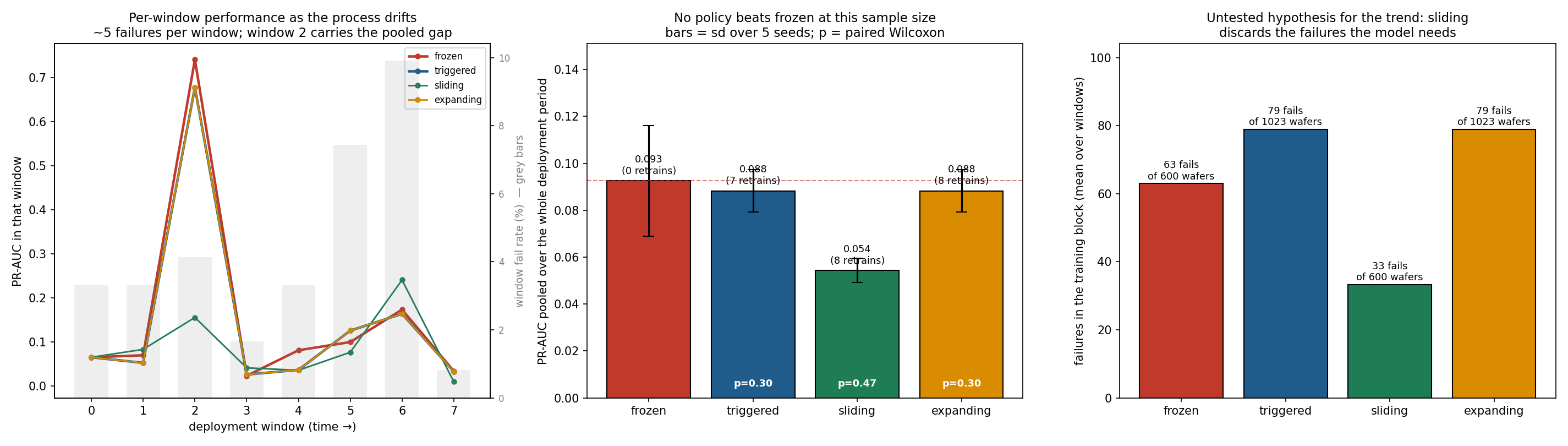
rolling_retrain.py simulates deployment: train on the first 600 wafers, then walk forward through 8 evaluation windows of ~120 wafers, comparing four policies at identical windows. Every retrain refits the column selection, imputation medians, scaler, model and decision threshold — nothing at window w may touch data from w onward.
| policy | PR-AUC (pooled) | capture@20% | retrains | failures in training block | vs frozen |
|---|---|---|---|---|---|
| frozen (train once, never again) | 0.093 | 0.346 | 0 | 63 of 600 | — |
| triggered (retrain on all history when PSI fires) | 0.088 | 0.337 | 7 | 79 of 1023 | −4.6% |
| expanding (retrain on all history every window) | 0.088 | 0.337 | 8 | 79 of 1023 | −4.6% |
| sliding (retrain on the most recent 600) | 0.054 | 0.224 | 8 | 33 of 600 | −41.3% |
No retraining policy beats leaving the model frozen. And the −41% on the
sliding window is not a finding — it is an artefact of pooling. Window 2
alone accounts for 75% of that gap and contains 5 failures. Compared
window by window with seeds averaged, sliding is 3–4 against frozen with
Wilcoxon p = 0.47; expanding and triggered are 2–5 with p = 0.30.
Nothing here is significant (outputs/rolling_retrain_paired_test.csv).
The honest conclusion is that SECOM cannot answer the retraining question. The deployment period holds 41 failures spread across 8 windows; that is not enough resolution to separate four policies. Reporting the pooled −41% as "retraining hurts" would have been exactly the mistake this repo keeps catching elsewhere.
Two things the experiment does establish:
- The PSI trigger fires in 7 of 8 windows. At a 10% action-band threshold the drift is so pervasive that "retrain when drift is detected" is operationally identical to "retrain every time" — it saves one retrain out of eight. A drift trigger buys no economy on this process.
- The policies differ enormously in how many failures they get to learn from — 33 (sliding) vs 63 (frozen) vs 79 (expanding). That is a plausible mechanism for the trend, and it suggests that under a rare positive class you should grow the training window rather than slide it. It is a hypothesis, not a result: the paired test cannot confirm it here.
What would answer the question: more failures per window. Either a longer deployment record or a process with a higher fail rate. The experiment is written to be re-pointed at either.
Decision guidance (explainability → actionability)
- With FN:FP = 100:1 at 6% prevalence, "inspect everything" is the cost floor — so the real constraint is inspection capacity, reported as capture@20%: fails caught if only the riskiest 20% of wafers can be re-inspected (XGBoost: 27% vs 20% random; modest, for the drift reasons above).
- SPC T² catches only 8% of fails at 11% false alarms: the fails are not global multivariate outliers, which justifies supervised ML over pure SPC.
- Threshold sits at the cost-curve minimum chosen on validation (dashed
lines in
figures/cost_vs_threshold.png), not at 0.5.
Why these metrics
- PR-AUC not ROC-AUC: at 6% prevalence ROC-AUC is inflated by the easy negatives. Accuracy is banned — predicting "all pass" scores 94%.
- Expected cost turns the confusion matrix into money, making threshold choice a business decision.
- capture@20% answers the operator's actual question: "I can re-check N wafers per shift — how many fails does that catch?"
Sensor correlation network (M4) — and why it changes nothing
sensor_network.py builds a correlation network over the 444 surviving sensors using the standard fMRI functional-connectivity recipe: correlate every pair, keep the strongest 5% of edges (proportional thresholding), rank nodes by degree centrality, call the top ones hubs. Fit on the training window only, since the network is part of the model.
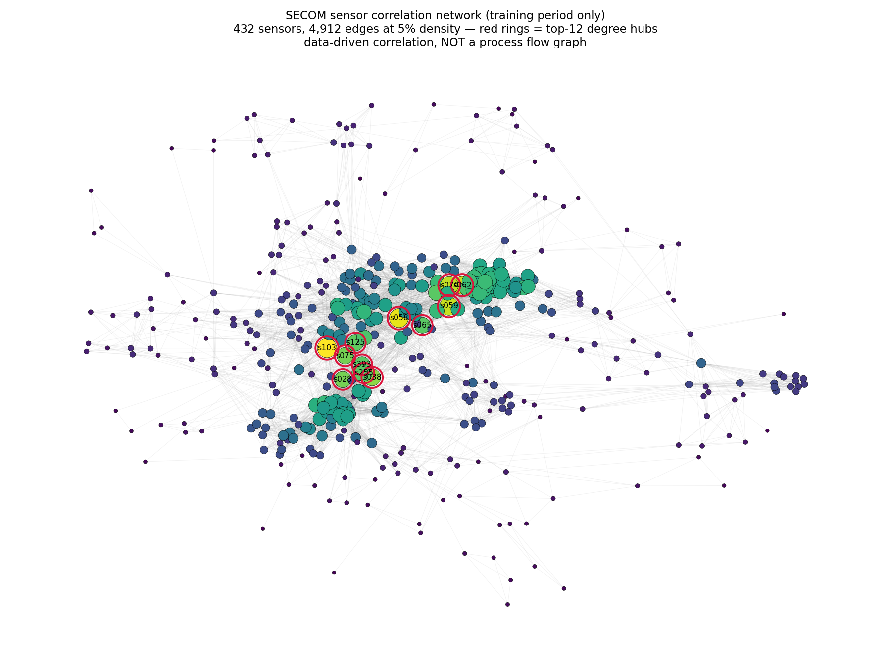
This is a data-driven correlation network, not a process flow graph. The sensors are anonymized; nothing here says which process step any of them belongs to. The genuine process-flow story lives in 03_bosch.
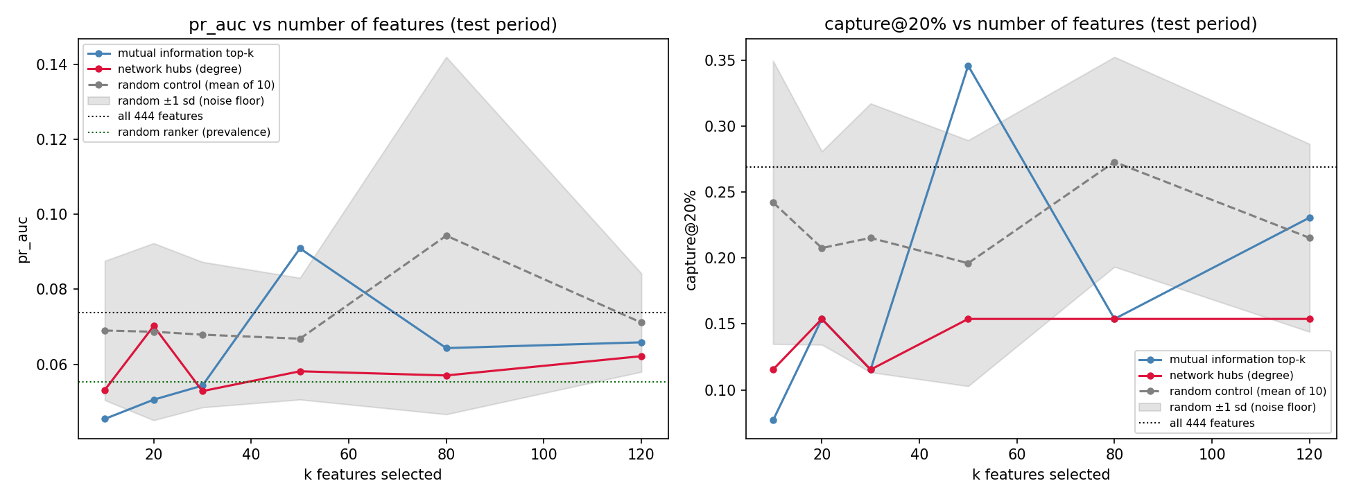
The network is real — s103, s058, s059 and s062 sit at 76–83 connections each, far above the rest. The useful question is whether hub-ness makes them better features, tested against mutual-information top-k and, critically, against randomly chosen subsets of the same size:
| k | network hubs | mutual info top-k | random control (mean ± sd) |
|---|---|---|---|
| 10 | 0.053 | 0.045 | 0.069 ± 0.019 |
| 20 | 0.070 | 0.051 | 0.069 ± 0.024 |
| 30 | 0.053 | 0.054 | 0.068 ± 0.019 |
| 50 | 0.058 | 0.091 | 0.067 ± 0.016 |
| 80 | 0.057 | 0.064 | 0.094 ± 0.048 |
| 120 | 0.062 | 0.066 | 0.071 ± 0.013 |
(PR-AUC on the test period; all 444 features scores 0.074.)
Neither principled method beats picking sensors at random. At every k, both sit inside ±1 sd of the random control, and nothing beats simply keeping all 444 features. The k=50 mutual-information value of 0.091 looks like a win until you notice the random control reaches 0.094 on its own at k=80.
Without the random control this section would have reported "network hub selection beats mutual information at k=20" and been wrong. With ~26 positive cases in the test window and the drift documented above, differences of this size are noise. The honest conclusion is that on SECOM the network is a description of the measurement system, not a feature-selection tool.
PHM 2016 CMP — Virtual Metrology (L2: in-process time series)
Business problem
Chemical-mechanical planarization polishes material off a wafer surface. Measuring how much came off — the material removal rate (MRR) — is slow, needs dedicated metrology capacity, and happens after the fact. Every wafer that has to be physically measured is a wafer occupying a metrology slot and a polishing result you learn too late to act on.
If the in-process sensor trace predicts MRR, that measurement can be skipped for most wafers and a bad polish can be caught during the run rather than after it. This is virtual metrology, and this is the one sub-project that is 100% semiconductor with genuine in-process time series.
Result
Evaluated on the official 424-run competition test set (not a self-made holdout — see "Recovering the withheld labels" below):
| model | test MSE | RMSE | MAE | R² |
|---|---|---|---|---|
| Baseline: training mean | 846.4 | 29.1 | 21.7 | 0.00 |
| Baseline: per-stage mean | 785.7 | 28.0 | 22.0 | 0.07 |
| Ridge (standardised) | 25.2 | 5.02 | 3.67 | 0.970 |
| RandomForest | 7.64 | 2.76 | 1.94 | 0.991 |
| XGBoost | 6.24 | 2.50 | 1.82 | 0.993 |
MSE is the competition's official metric, so these are directly comparable to the published 2016 results. A mean absolute error of 1.8 on removal rates spanning 57–160 is roughly 2% error — inside the range where virtual metrology can genuinely displace physical measurement for routine wafers.
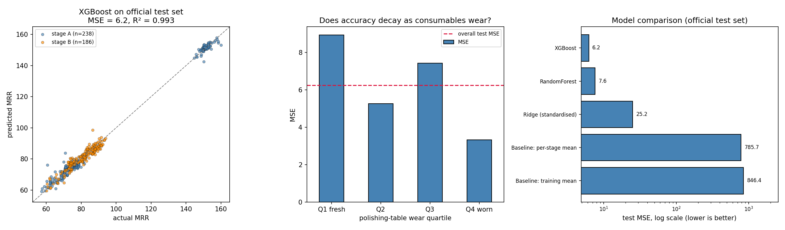
The R² is partly an illusion, and here is the honest number
MRR is strongly bimodal: a dense cluster around 75 and a separate cluster
around 150, with almost nothing between (figures/eda_mrr_and_wear.png).
Telling those two clusters apart is easy, and it inflates R² across the full
range. Restricted to the main cluster (MRR < 120, 351 of 424 test runs), the
same model scores R² = 0.897, MSE 6.80, MAE 1.93. That is the number that
reflects actual metrology precision, and it is the one worth quoting.
Recovering the withheld labels
The challenge closed in 2016 with test labels withheld — the official
CMP-test-removalrate.csv ships with ? in every row — and
phmsociety.org now 404s on its own download links. Two steps unblocked it:
- The data itself is preserved in the Internet Archive;
download_data.pyfalls back to the archived snapshots automatically. - The test labels were separately published on Kaggle as
markshizhe/cmp-data-set. That file is 5.6 KB and useless on its own — no trajectories, no training data — but its 424(WAFER_ID, STAGE)keys match the official test key set exactly, 100%, with real numeric MRR values in place of the?.
Joining the two gives an honest evaluation on the real competition test set.
Method
- Assembly (
prepare.py) — 185 CSVs → 672,744 trajectory rows → 1,981 runs, each a(WAFER_ID, STAGE)pair with a few hundred samples of 19 process signals. Test: 156,262 rows → 424 runs. - Data quality — 4 training runs report MRR of 200–4,326 against a median of 79 and a 99.5th percentile of 160. They are dropped as corrupt. The bound is set from the training distribution alone; the test range was not consulted, so this is not test peeking.
- Features (
features.py) — per signal: level, spread, extremes, trend (slope), shape (skew/kurtosis), endpoints, plus frequency-domain descriptors (spectral centroid, low-band energy share, spectral entropy). Runs vary in length, so every feature is length-invariant. Consumable-usage channels are summarised by level — they are the tool-wear state, not a trajectory. 208 features from 19 signals. - Split —
group_temporal_splitonWAFER_ID, ordered by run start time. A wafer's stage A and stage B runs always land on the same side; the split asserts wafer-disjointness rather than trusting it.
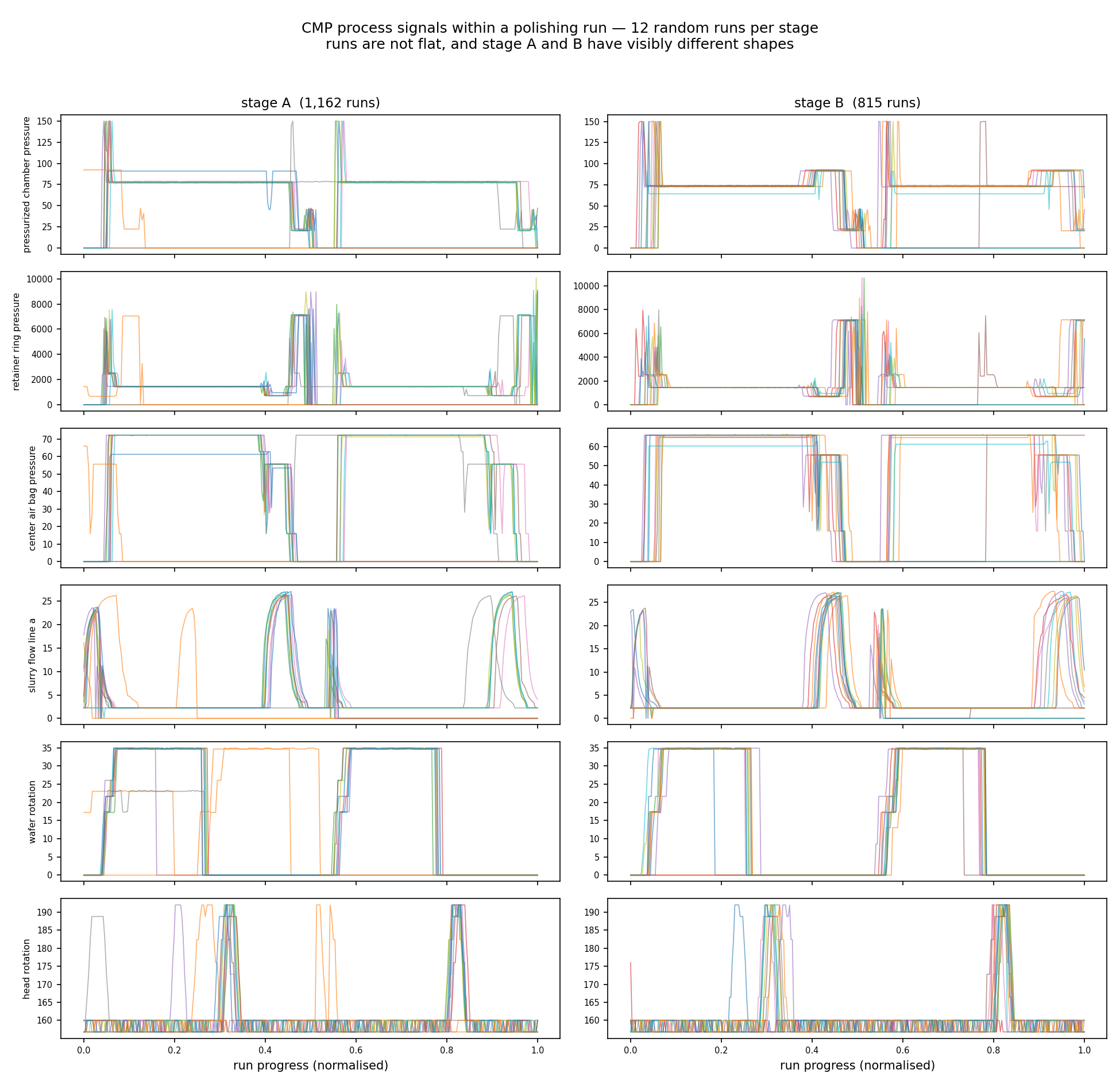
The trajectories are what justify the whole L2 layer: runs are multi-phase polishing recipes with distinct step structure, and stage A and stage B have visibly different phase patterns. If runs were flat, per-run averages would suffice and this would just be another tabular problem.
Tool ageing: the hypothesis is not supported, and that is reported
The spec's expectation was that error grows as the polishing pad and dresser wear, motivating a retraining trigger. Stratifying test error by polishing-table usage quartile:
| wear quartile | n | MSE | bias | MAE |
|---|---|---|---|---|
| Q1 fresh | 106 | 8.93 | +0.47 | 2.16 |
| Q2 | 106 | 5.27 | −0.12 | 1.79 |
| Q3 | 106 | 7.43 | +0.62 | 1.90 |
| Q4 worn | 106 | 3.32 | +0.15 | 1.44 |
Error does not grow with wear — the worn quartile is the most accurate. Because usage is an input feature, the model has already learned the wear effect rather than being degraded by it. The retraining trigger for this process should therefore watch for novel operating conditions (usage values outside the trained range, recipe changes), not accumulated hours. Per stage, errors are comparable (A: 6.00, B: 6.53).
This is the opposite of what SECOM and Bosch show, and the contrast is the point: drift is not automatic. Here the degradation axis was measured and fed to the model, so it stopped being drift.
Reproducing
python 02_phm_cmp/download_data.py     # falls back to Internet Archive
python 02_phm_cmp/prepare.py
python 02_phm_cmp/plot_trajectories.py
python 02_phm_cmp/run_model.py
python 02_phm_cmp/sequence_models.py   # ~40 min on CPU
download_data.py retrieves the trajectories, but the recovered test labels
must be placed at 02_phm_cmp/data/CMP-test-removalrate_recovered.csv
(columns WAFER_ID, STAGE, AVG_REMOVAL_RATE) from the Kaggle dataset above.
Traps avoided
- A wafer never straddles the split. Its stage A and stage B runs share a wafer and much of their context; splitting rows at random would leak.
- No global scaling. Ridge's imputer and scaler sit inside a pipeline fit on training folds only.
- Length-invariant features. Runs differ in sample count; raw concatenation or fixed-index features would encode run length as signal.
- R² reported twice. Once across the full bimodal range, once within the main cluster, because the first number flatters the model.
Hand-crafted features vs learned representations (M4)
Track 2 (sequence_models.py) puts a 1D-CNN and a bidirectional GRU on the raw trajectories, resampled onto a common 0–1 progress axis. Everything else is held identical to track 1 — same group-aware split, same official test set, same metric, same static inputs (tool wear, stage, chamber, run length). Only the trajectory encoding differs. Each architecture is run with 3 seeds and ensembled, because at this sample size a single run is a coin flip.
| model | track | val MSE | test MSE | test MAE | test R² |
|---|---|---|---|---|---|
| XGBoost | hand-crafted | 31.98 | 6.24 | 1.82 | 0.993 |
| RandomForest | hand-crafted | 29.57 | 7.64 | 1.94 | 0.991 |
| BiGRU (3 seeds) | learned | 27.63 | 14.45 | 2.80 | 0.983 |
| Ridge | hand-crafted | 44.47 | 25.17 | 3.67 | 0.970 |
| 1D-CNN (3 seeds) | learned | 18.01 | 28.59 | 3.23 | 0.966 |
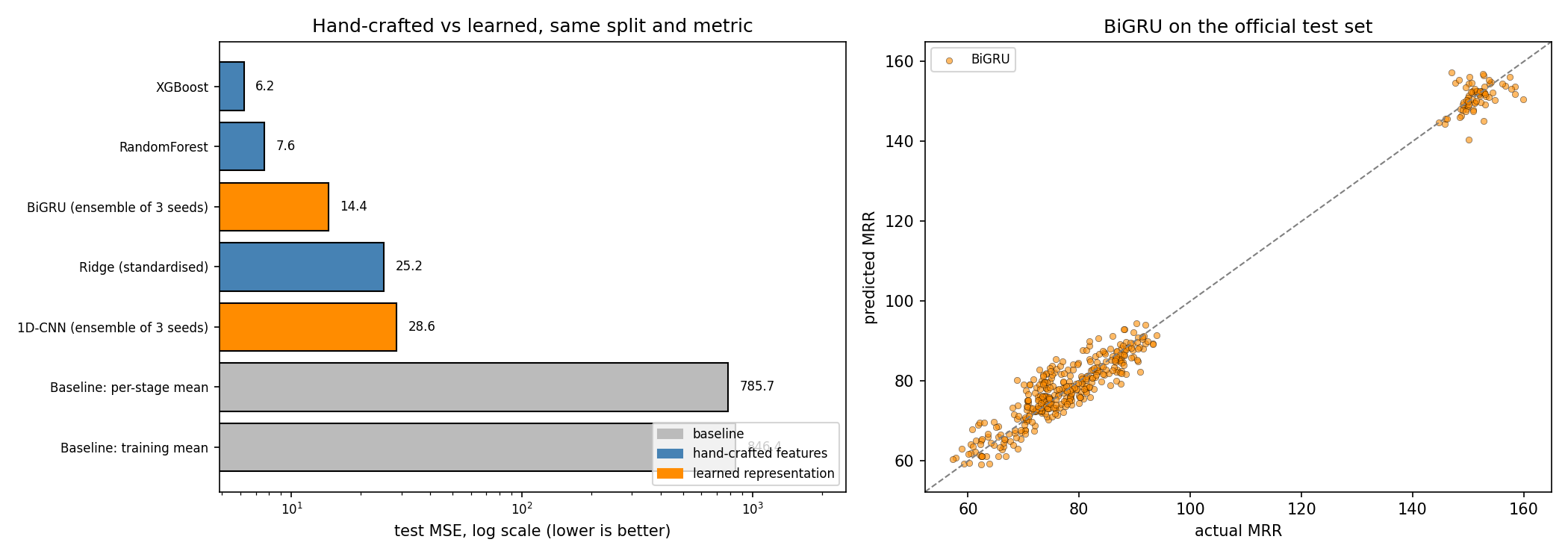
Hand-crafted features win by 2.3× (6.24 vs 14.45). At n ≈ 1,600 training runs, compressing a trajectory into ~200 physically-motivated descriptors and letting a tree model sort them out beats asking a network to discover the same structure from scratch.
The sharper lesson is in the validation column. The 1D-CNN has the best validation MSE of any model here (18.01) and the worst test MSE of any non-baseline model (28.59). Its ranking is exactly inverted between the two. Its seed spread is 26.7–39.8 — a 49% swing — while the GRU's is 14.9–15.8. That is what overfitting to a 398-run validation set looks like: had I selected on validation and reported a single seed, I would have shipped the worst model and called it the best.
So the answer to "which would you choose?" is not a preference, it is a sample-size argument: below a few thousand runs, hand-crafted time and frequency features plus a tree are the safer bet, and the deep model's apparent validation win is exactly the signal you should distrust.
Bosch — From Predicting Failures to Locating Them (L3: process graph)
⚠️ Honest framing: Bosch is automotive, not semiconductor. It is used here because it is the public dataset whose schema encodes a complete production-line structure, which is what makes graph methods demonstrable at all. A wafer fab's process flow has the same shape — stations, routes, per-station metrology — so the method transfers even though the parts don't. Public semiconductor data is almost always anonymized (see SECOM), which is precisely why the graph story has to be told here.
Business problem
1.18M products cross up to 23 of 52 stations on 4 production lines. 0.58% fail final quality control. Catching them matters, but knowing where they were damaged matters more: a prediction tells you to scrap one part, an attribution tells you which station to go fix. The cost asymmetry (an escaped defect reaching a customer vs. pulling a good part for inspection) is taken as 50:1.
The graph is reconstructed, not given
Nothing in the data says "these stations are connected". The structure comes from two places:
- Column names —
L3_S36_F3939= line 3, station 36, feature 3939. Parsed in structure.py (unit-tested in tests/test_bosch_structure.py). - Date columns — the timestamp at each station gives the order a product visited them, and therefore the edges.
That yields 52 stations, 243 distinct transitions, and 7,927 distinct production paths, with a median of 13 stations visited per product.
Result 1 — attribution works, and it points at one station
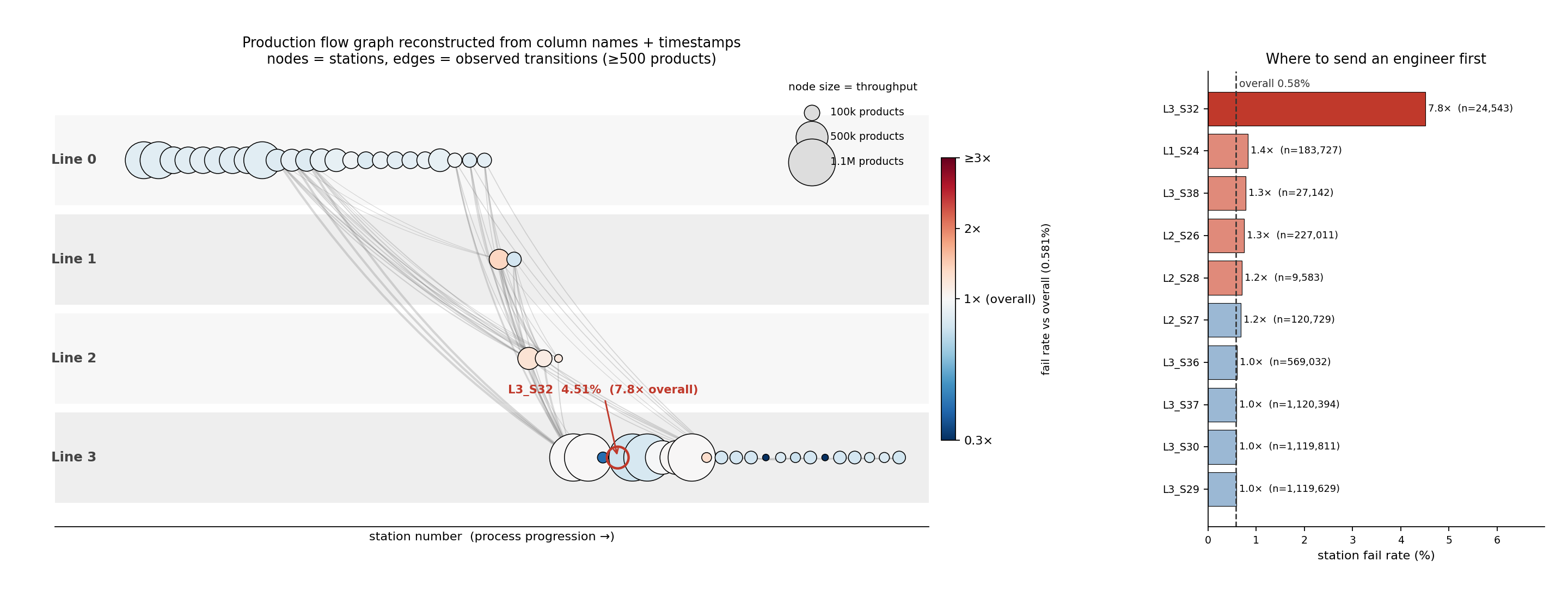
L3_S32 fails at 4.51%, 7.8× the 0.58% overall rate, across 24,543
products. No other station exceeds 1.5×. That is a concrete, checkable,
send-an-engineer-tomorrow finding, and it comes from the graph, not the model
(outputs/station_attribution.csv).
Path-level attribution agrees: products routed L1_S24 → L3_S29 (skipping
the L2 inspection stations entirely) fail at 1.28%, roughly double the 0.67%
of the otherwise-identical route that passes through L2_S26
(outputs/paths_highest_fail_rate.csv).
The SPC baseline, and why it cannot work on a multi-route plant
Before claiming ML is needed, run the chart a process engineer would reach for. Hotelling T² compares a unit's measurement vector to an in-control mean and covariance — which presumes every unit is measured the same way. With 7,927 distinct routes, most measurement slots are empty for most products, and those blanks are stations never visited, not readings that went missing.
So spc_baseline.py runs the chart twice:
| baseline | n test | recall @UCL | false alarms | PR-AUC | random |
|---|---|---|---|---|---|
| T² over all products (median-imputed) | 354,950 | 46.1% | 35.9% | 0.0047 | 0.0039 |
| T² within the largest route family | 8,755 | 6.5% | 5.2% | 0.0051 | 0.0035 |
| XGBoost model A, for comparison | 354,950 | — | — | 0.0244 | 0.0039 |
The naive chart's 46% recall is an illusion: it comes from alarming on more than a third of all good products, and its PR-AUC is 1.2× random — essentially no ranking power. Imputation made routing differences look like process excursions.
Restricted to the largest route family (58,379 products sharing 24 measurement columns), where the assumption genuinely holds, T² is legitimate and scores 1.5× random. Still negligible.
That is the honest bar: SPC runs at 1.2–1.5× random here, ML at 6.2×. And the reason SPC fails is structural rather than statistical — the plant does not have one process to chart, it has 7,927 of them. Which is precisely the argument for modelling the routing explicitly.
Result 2 — the graph features do not improve prediction, and that is the interesting part
Ablation under one temporal split (fit 650,740 / val 177,475 / test 354,950, split on each product's first timestamp; 582 products with no timestamp at all are dropped rather than silently sorted into test):
| model | MCC @val thr | MCC @oracle thr | PR-AUC | capture@20% | capture@5% | recall@1%FPR |
|---|---|---|---|---|---|---|
| A: station aggregates + routing | 0.069 | 0.112 | 0.024 | 0.287 | 0.165 | 0.129 |
| B: + path & graph features | 0.099 | 0.102 | 0.018 | 0.272 | 0.144 | 0.107 |
| C: GNN on routing subgraphs | 0.062 | 0.095 | 0.018 | 0.260 | 0.122 | 0.086 |
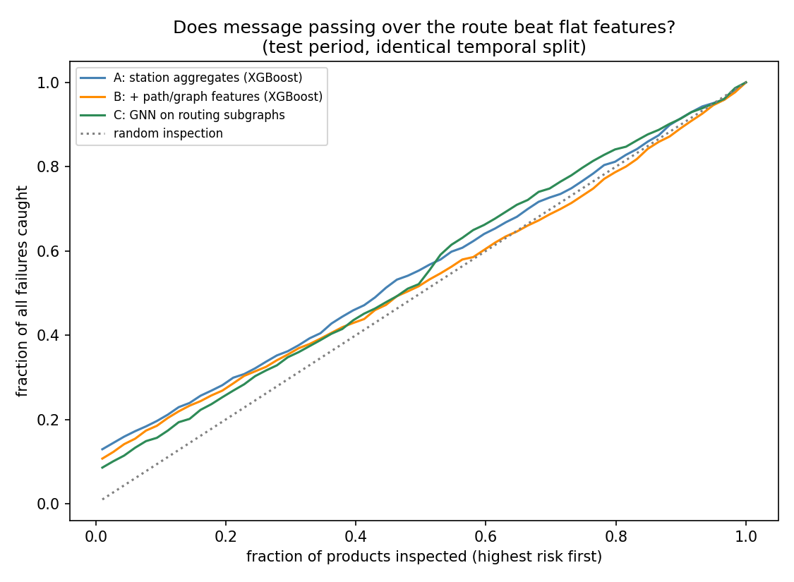
Read only the first column and the graph features look like a 43% MCC win. They are not. MCC depends on a threshold, and at the oracle threshold — the best any of them could possibly achieve on test — model A is ahead (0.112 vs 0.102 vs 0.095). Model B's apparent gain was its validation threshold happening to land closer to its test optimum. Every threshold-free metric (PR-AUC, capture, recall@1%FPR) says the plain tabular model A ranks best.
Model C (run_gnn.py) injects the structure a second, entirely different way: each product becomes a subgraph whose nodes are the stations it visited, with that station's readings as node features and its route as the edges, so message passing can combine a reading with its neighbours' along the route. It lands with model B, behind A. Two independent ways of adding the graph, same answer.
That gap between MCC@val (0.069) and MCC@oracle (0.112) for model A is worth its own note: even the threshold does not transfer across time here, because prevalence moves (0.75% → 0.33% → 0.40% across the three windows).
XGBoost loves the graph block — path_risk ranks first by gain, ahead
of every station measurement (figures/attribution_importance.png). Yet it
makes the model worse. Importance measures what a model leaned on, not
whether leaning helped.
One fairness note that changed the GNN's numbers materially: training is subsampled (25 negatives per failure — 1.18M products is far more than a CPU GNN needs), but validation and test are kept at full prevalence. An earlier run picked thresholds on a subsampled validation set at 3.85% positives and they did not transfer to a 0.40% test set, inflating cost per part 5×. Thresholds have to be chosen at the prevalence they will face.
The diagnosis is in diagnose_encoding.py:
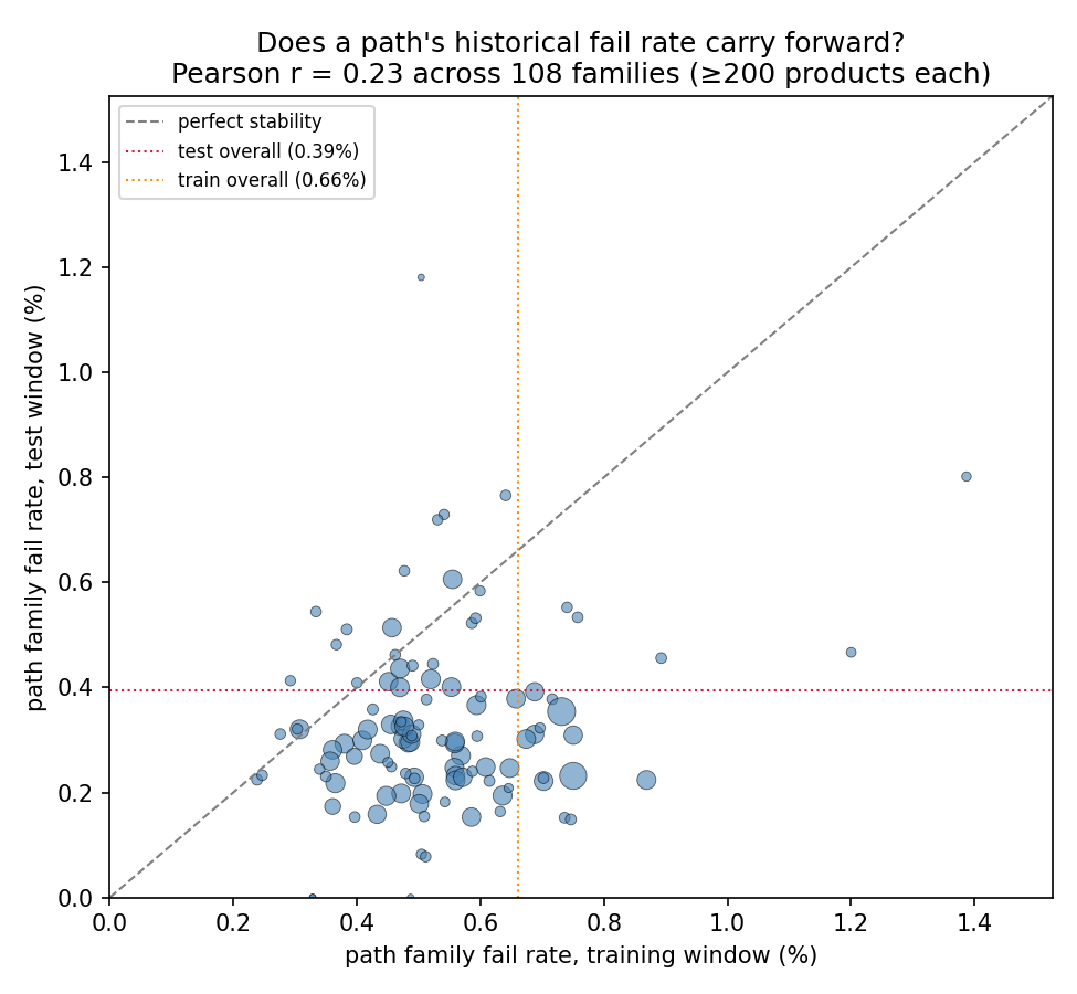
- Of 108 path families with ≥200 products in both windows, the correlation between a family's training fail rate and its test fail rate is Pearson r = 0.23, Spearman ρ = 0.09 (p = 0.36 — not significant).
- This is not a cold-start problem: 99.2% of test products belong to a path family seen in training.
- The whole factory drifts: overall fail rate falls 0.66% → 0.40% between the two windows — the same yield-ramp pattern SECOM shows.
- And it is not only the labels. Running the same PSI monitor SECOM uses
(
common/drift.py) over the 50 station-level means: median PSI 0.183, with 20 of 50 in the action band (L3_S44, L3_S43, L0_S4 worst). The retraining trigger fires here too (outputs/feature_drift_psi.csv).
So a path's historical fail rate is a level the model memorises, not a property of the route. Target-encoding it looks brilliant in cross-validated importance and quietly degrades out-of-time ranking. The graph earns its keep as an attribution instrument, not as a feature generator — which is the honest answer to "what does the graph give you that a tabular model doesn't?"
Deliberately not done: the "magic features"
Public Bosch solutions reach MCC ≈ 0.4+ largely via leakage artefacts — row
Id ordering correlates with the response because the file was sorted with
label-adjacent information. Those features are excluded here. The numbers
below are what the process data actually supports; the point of this
sub-project is method, not leaderboard position.
Reproducing
python 03_bosch/download_data.py    # needs ~/.kaggle/kaggle.json + accepted rules
python 03_bosch/prepare.py          # chunked reduction, ~6 min, writes cache/
python 03_bosch/build_graph.py      # graph, attribution tables, flagship figure
python 03_bosch/run_model.py        # A/B ablation
python 03_bosch/diagnose_encoding.py
train_numeric.csv and train_date.csv total 4.7 GB, so prepare.py reads
them in 100k-row chunks and collapses ~2,100 columns to per-station
aggregates before anything is held in memory at once.
Traps avoided
- Missing ≠ missing measurement. A null usually means "this product never
visited this station", which is routing information, not a gap to impute.
It is preserved as
{station}__n(readings taken) and left as NaN for XGBoost to split on natively — never imputed. - No random splitting. Split on the product's first timestamp.
- No label leakage into encodings. Station- and path-risk encodings are computed on the fit window only, smoothed toward the prior.
- No accuracy, ever. At 0.58% positives, predicting "all pass" scores 99.4%. Reported: MCC (competition metric), PR-AUC, and decile capture.